So, you’ve been working with MySQL for a while and now are being asked to manage it. Perhaps your primary job description is not about support and maintenance of the company’s databases (and data!), but now you’re expected to properly maintain one or more MySQL instances. It is not uncommon that developers, or network/system administrators, or DevOps folks with general backgrounds, find themselves in this role at some point in their career.
So, what does a DBA do? We know that a DBA manages the company’s databases, what does that mean? In this series of posts, we’ll walk you through the daily database operations that a DBA does (or at least ought to!).
We plan on covering the following topics, but do let us know if we’ve missed something:
- Monitoring tools
- Trending
- Periodical healthchecks
- Backup handling
- High Availability
- Common operations (online schema change, rolling upgrades, query review, database migration, performance tuning)
- Troubleshooting
- Recovery and repair
- anything else?
In today’s post, we’ll cover monitoring and trending.
Monitoring and Trending
To manage your databases, you would need good visibility into what is going on. Remember that if a database is not available or not performing, you will be the one under pressure so you want to know what is going on. If there is no monitoring and trending system available, this should be the highest priority. Why? Let’s start by defining ‘trending’ and ‘monitoring’.

A monitoring system is a tool that keeps an eye on the database servers and alerts you if something is not right, e.g., a database is offline or the number of connections crossed some defined threshold. In such case, the monitoring system will send a notification in some defined way. Such systems are crucial because, obviously, you want to be the first to be informed if something’s not right with the database.
On the other hand, a trending system will be your window to the database internals. It will provide you with graphs that show you how those cogwheels are working in the system - the number of queries per second, how many read/write operations the database does on different levels, are table locks immediate or do queries have to wait for them, how often a temporary table is created, how often it is created on disk, and so on. If you are familiar with MySQL internals, you’ll be better equipped to analyze the graphs and derive useful information. Else, you may need some time to understand these graphs. Some metrics are pretty self-explanatory, others perhaps not so obvious. But in general, it’s probably better to have more data than not to have any when it’s needed.
Data is presented as graphs for better visibility - from graphs, the human mind can easily derive trends and locate anomalies. The trending system also gives you an idea of how things change over time - you need this visibility in both real time and for historical data, as things happen also when people sleep. If you have been on-call in an ops team, it is not unusual for an issue to have disappeared by the time you get paged at 3am, wake up, and log into the system.
Monitoring - best practices
There are many many monitoring solutions out there, chances are you probably have one of the following options already in your infrastructure:
Nagios:

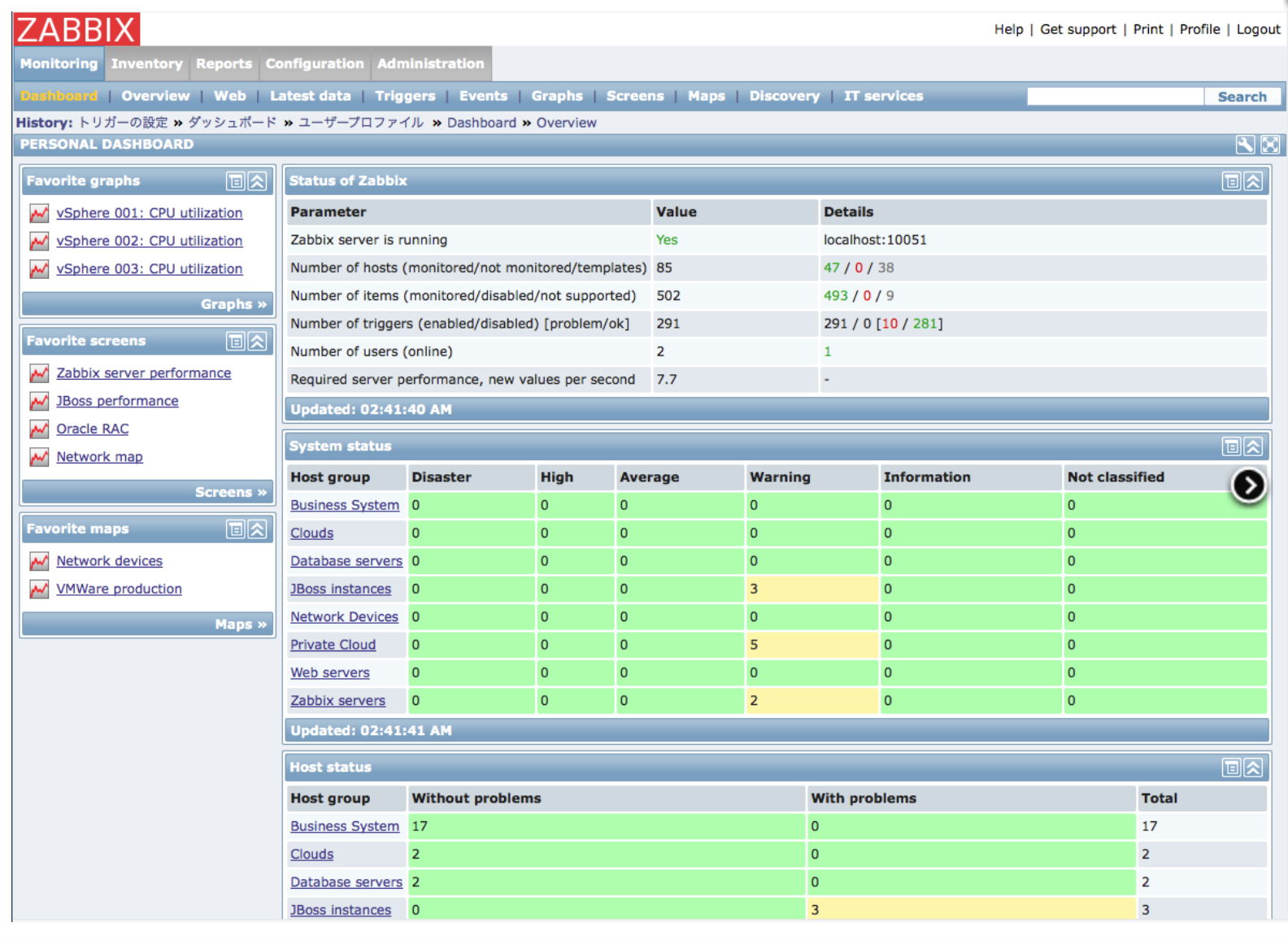
Zabbix:
MONyog:

ClusterControl:

All of those tools have their pros and cons. Some are only for monitoring, others also provide you with trending. A good monitoring system should allow you to customize the thresholds of alerts, their severity, etc., and fine-tune it to your own needs. You should also be able to integrate with external paging services like PagerDuty.
How you’d like your monitoring setup to look like is also up to individual preferences. What we’d suggest is to focus on the most important aspects of your operations. As a general rule of thumb, you’d be interested to know if your system is up or not, if you can connect to the database, whether you can execute meaningful read and write queries (ideally something as close to the real workload as possible, for example you could read from a couple of production tables). Next in the order of importance would be to check if there’s an immediate threat to the system’s stability - high CPU/memory/disk utilization, lack of disk space. You want to have your alerts as actionable as possible - being waken up in the middle of the night, only to find that you can’t do anything about the alert, can be frustrating in the long run.
Trending - best practices
Next step would be to install some trending software. Again, similar to the monitoring tools, there is a plethora of choices. Best known are Cacti:

Munin:

and Zabbix:

ClusterControl, in addition to the cluster management, can also be used as a trending system.

There are also SaaS-based tools including Percona Cloud Tools and VividCortex.
Having a trending solution is not enough - you still have to know what kind of graphs you need. MySQL-focused monitoring tools will work great as they are focused on MySQL - they were created to bring to the MySQL DBA as much information as possible. Other tools that are of more generic nature will probably have to be configured. It would be outside the scope of this blog to go over such configurations, but we’d suggest to look at Percona Monitoring Plugins. They are prepared for Cacti and Zabbix (when it comes to trending) and you can easily set them up if you have chosen one of those tools. If not, you can still use them as a guide as to what MySQL metrics you want to have graphed and how to do that.
Once you have both monitoring and trending tools ready, you can go to the next phase - gathering the rest of the tools you will need in your day-to-day operations
CLI tools
In this part, we’d like to cover some useful CLI tools that you may want to install on your MySQL server. First of all, you’ll want to install Percona Toolkit. It is a set of tools designed to help DBAs in their work. Percona Toolkit covers tasks like checking data consistency across slaves, fixing data inconsistency, performing slow query audits, checking duplicate keys, keeping track of configuration changes, killing queries, checking grants, gathering data during incidents and many others. We will be covering some of those tools in the coming blogs, as we discuss different situations a DBA may end up into.
Another useful tool is sysbench. This is a system benchmarking tool with an OLTP test mode. That test stresses MySQL and allows you to get some understanding of the system’s capacity. You can install it by running apt-get/yum but you probably want to make sure that you have version 0.5 available - it included support for multiple tables and the results are more realistic. If you’d like to perform more detailed tests and closer to your “real world” workload, then take a look at Percona Playback - this tool can use “real world” queries in form of a slow query log or tcpdump output and then replay those queries on the test MySQL instance. While it might sound strange, performing such benchmarks to tune a MySQL configuration is not uncommon, especially at the beginning when a DBA is learning the environment. Please keep in mind that you do not want to perform any kind of benchmarking (especially with Percona Playback) on the production database - you’ll need a separate instance setup for that.
Jay Janssen’s myq_gadgets is another tool you may find useful. It is designed to provide information about the status of the database - statistics about com_* counters, handlers, temporary tables, InnoDB buffer pool, transactional logs, row locking, replication status. If you are running Galera cluster, you may benefit from ‘myq_status wsrep’ which gives you nice insight into writeset replication status including flow control.
At some point you’ll need to perform a logical dump of your data - it can happen earlier, if you already make logical backups, or later - when you’ll be upgrading your MySQL to a new major version. For larger datasets mysqldump is not enough - you may want to look into a pair of tools: mydumper and myloader. Those tools will work together to create a logical backup of your dataset and then load it back to the database. What’s important - they can utilize multiple threads which speeds up the process significantly compared to mysqldump. Mydumper needs to be compiled and it’s sometimes hard to get it to work. Recent versions became more stable though and we’ve been using it successfully.
Periodical health checks
Once you have all your tools set up, you need to establish a routine to check the health of the databases. How often you’d like to do it is up to you and your environment. For smaller setups daily checks may work. For larger setups you probably have to do it every week or so. The reasoning behind it is that such regular checks should enable you to act proactively and fix any issues before they actually happen. Of course, you will eventually develop your own pattern but here are some tips on what you may want to look at.
First of all, the graphs! This is one of the reasons a trending system is so useful. While looking at the graphs, you want to ensure no anomalies happened since the last check. If you noticed any kind of spikes, drops or, in general, unusual patterns, you probably want to investigate further to understand what happened exactly. It’s especially true if the pattern is not healthy and may be the cause (or result) of a temporary slowdown of the system.
You want to look at the MySQL internals and host stats. Most important graphs would be the ones covering number of queries per second, handler statistics (which gives you information about how MySQL accesses rows), number of connections, number of running connections, I/O operations within InnoDB, data about row and table level locking. Additionally, you’re interested in all data on host level - CPU utilization, disk throughput, memory utilization, network traffic. See the “Related resources” section at the end of this post for a list of relevant blogs around monitoring metrics and their meaning. At first, such a check may take a while but once you get familiar with your workload and its patterns, you won’t need as much time as at the beginning.
Another important part of the health check is going over the health of your backups. Of course, you might have backups scheduled. Still, you need to make sure that the process works correctly, your backups are actually running and backup files are created. We are not talking here about recovery tests (such tests should be performed but it’s not really required to do it daily or on weekly basis - on the other hand, if you can afford to do it, it’s even better). What we are talking here is more about simple checks. If the backup file was created, does it have the correct file size (if a data set has 100GB, then a 64KB backup file may be suspicious)? Has it been even created in the first place? If you use compression and you have some disk space free, you may want to try and decompress the archive to verify it’s correct (as long as it’s feasible in terms of the time needed for decompression). How’s the disk space status? Do you have enough free disk on your backup server? If you copy backups to a remote site for DR purposes, the same set of checks apply for the DR site.
Finally, you probably want to look at the system and MySQL logs - check kernel log for any symptoms of hardware failure (disk or memory sometimes send warning messages before they fail), check MySQL’s error log to ensure nothing wrong is going on.
As we mentioned before, the whole process may take a while, especially at the beginning. Especially the graph overview part may take time, as it’s not really possible to automate it - the rest of the processes is rather straightforward to script. With a growing number of MySQL servers, you will probably have to relax the frequency between checks due to time needed to perform a health check - maybe you’ll need to prioritize, and cover the less important parts of your infrastructure every other week?
Such healthcheck is a really useful tool for a DBA. We mentioned already that it helps to proactively fix errors before they start to create an issue, but there’s one more important reason. You might not always up to date when it comes to the new code that has been introduced in production. In the ideal world, each SQL code would have been reviewed by a DBA. In the real world, though, it’s rather uncommon. As a result of that, it may happen that the DBA is surprised by new workload patterns that start showing up. The good thing is that, once they are spotted, the DBA can work with developers to fix or optimize schemas and SQL queries. Health checks are one of the best tools to catch up on such changes - without them, a DBA would not be aware of bad code or database design that may eventually lead to a system outage.
We hope this short introduction will give you some information on how you may want to setup your environment and what tools you may want to use. We also hope that the first health checks will give you a good understanding of your system’s performance and help you understand any pain points that may already be there. In our next post, we will cover backups.
Related resources
- Blog - Monitoring Host Metrics of your Database Instances - How to interpret Operating System Data
- Blog - Monitoring Galera Cluster for MySQL or MariaDB - Understanding metrics and their meaning
- Blog - Monitoring Galera/MySQL/MariaDB - Understanding and Optimizing CPU-related InnoDB metrics
- Blog - Monitoring Galera/MySQL/MariaDB - Understanding and Optimizing IO-related InnoDB metrics
- Webinar replay - Deep dive into Galera monitoring (Galera Cluster for MySQL/MariaDB, Percona XtraDB Cluster)
Blog category:

PlanetMySQL Voting: Vote UP / Vote DOWN

 The MariaDB project is pleased to announce the immediate availability of


 However the developer was not sure how to begin.


