This blog post gives an introduction to resource groups in MySQL 8 and dynamical allocation to threads, as well as a related bug report.
↧
MySQL 8 Resource Group – introduction and dynamic allocation
↧
Monitoring Processes with Percona Monitoring and Management

A few months ago I wrote a blog post on How to Capture Per Process Metrics in PMM. Since that time, Nick Cabatoff has made a lot of improvements to Process Exporter and I’ve improved the Grafana Dashboard to match.
I will not go through installation instructions, they are well covered in original blog post. This post covers features available in release 0.4.0 Here are a few new features you might find of interest:
Used Memory
Memory usage in Linux is complicated. You can look at resident memory, which shows how much space is used in RAM. However, if you have a substantial part of process swapped out because of memory pressure, you would not see it. You can also look at virtual memory–but it will include a lot of address space which was allocated and never mapped either to RAM or to swap space. Especially for processes written in Go, the difference can be extreme. Let’s look at the process exporter itself: it uses 20MB of resident memory but over 2GB of virtual memory.


Meet the Used Memory dashboard, which shows the sum of resident memory used by the process and swap space used:

There is dashboard to see process by swap space used as well, so you can see if some processes that you expect to be resident are swapped out.
Processes by Disk IO

Processes by Disk IO is another graph which I often find very helpful. It is the most useful for catching the unusual suspects, when the process causing the IO is not totally obvious.
Context Switches
Context switches, as shown by VMSTAT, are often seen as an indication of contention. With contention stats per process you can see which of the process are having those context switches.

Note: while large number of context switches can be a cause of high contention, some applications and workloads are just designed in such a way. You are better off looking at the change in the number of context switches, rather than at the raw number.
CPU and Disk IO Saturation
As Brendan Gregg tells us, utilization and saturation are not the same. While CPU usage and Disk IO usage graphs show us resource utilization by different processes, they do not show saturation.

For example, if you have four CPU cores then you can’t get more than four CPU cores used by any process, whether there are four or four hundred concurrent threads trying to run.
While being rather volatile as gauge metrics, top running processes and top processes waiting on IO are good metrics to understand which processes are prone to saturation.
These graphs roughly provide a breakdown of “r” and “b” VMSTAT columns per process
Kernel Waits
Finally, you can see which kernel function (WCHAN) the process is sleeping on, which can be very helpful to access processes which are not using a lot of CPU, but are not making much progress either.
I find this graph most useful if you pick the single process in the dashboard picker:

In this graph we can see sysbench has most threads sleeping in
unix_stream_read_genericwhich corresponds to reading the response from MySQL from UNIX socket – exactly what you would expect!
Summary
If you ever need to understand what different processes are doing in your system, then Nick’s Process Exporter is a fantastic tool to have. It just takes few minutes to get it added into your PMM installation.
If you enjoyed this post…
You might also like my pre-recorded webinar MySQL troubleshooting and performance optimization with PMM.
The post Monitoring Processes with Percona Monitoring and Management appeared first on Percona Database Performance Blog.
↧
↧
Custom Graphs to Monitor your MySQL, MariaDB, MongoDB and PostgreSQL Systems - ClusterControl Tips & Tricks

Graphs are important, as they are your window onto your monitored systems. ClusterControl comes with a predefined set of graphs for you to analyze, these are built on top of the metric sampling done by the controller. Those are designed to give you, at first glance, as much information as possible about the state of your database cluster. You might have your own set of metrics you’d like to monitor though. Therefore ClusterControl allows you to customize the graphs available in the cluster overview section and in the Nodes -> DB Performance tab. Multiple metrics can be overlaid on the same graph.
Cluster Overview tab
Let’s take a look at the cluster overview - it shows the most important information aggregated under different tabs.
Cluster Overview Graphs
You can see graphs like “Cluster Load” and “Galera - Flow Ctrl” along with couple of others. If this is not enough for you, you can click on “Dash Settings” and then pick “Create Board” option. From there, you can also manage existing graphs - you can edit a graph by double-clicking on it, you can also delete it from the tab list.
Dashboard Settings
When you decide to create a new graph, you’ll be presented with an option to pick metrics that you’d like to monitor. Let’s assume we are interested in monitoring temporary objects - tables, files and tables on disk. We just need to pick all three metrics we want to follow and add them to our new graph.
New Board 1
Next, pick some name for our new graph and pick a scale. Most of the time you want scale to be linear but in some rare cases, like when you mix metrics containing large and small values, you may want to use logarithmic scale instead.
New Board 2
Finally, you can pick if your template should be presented as a default graph. If you tick this option, this is the graph you will see by default when you enter the “Overview” tab.
Once we save the new graph, you can enjoy the result:
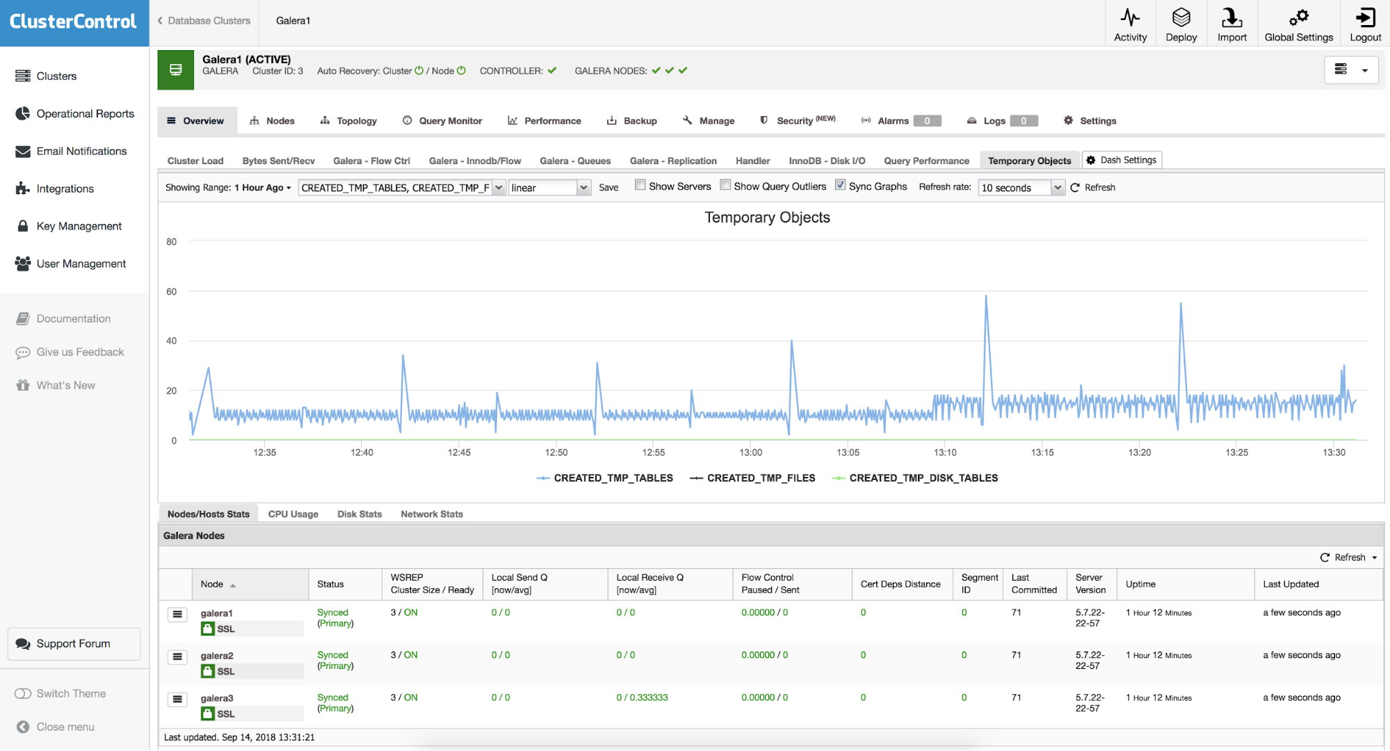
New Board 3
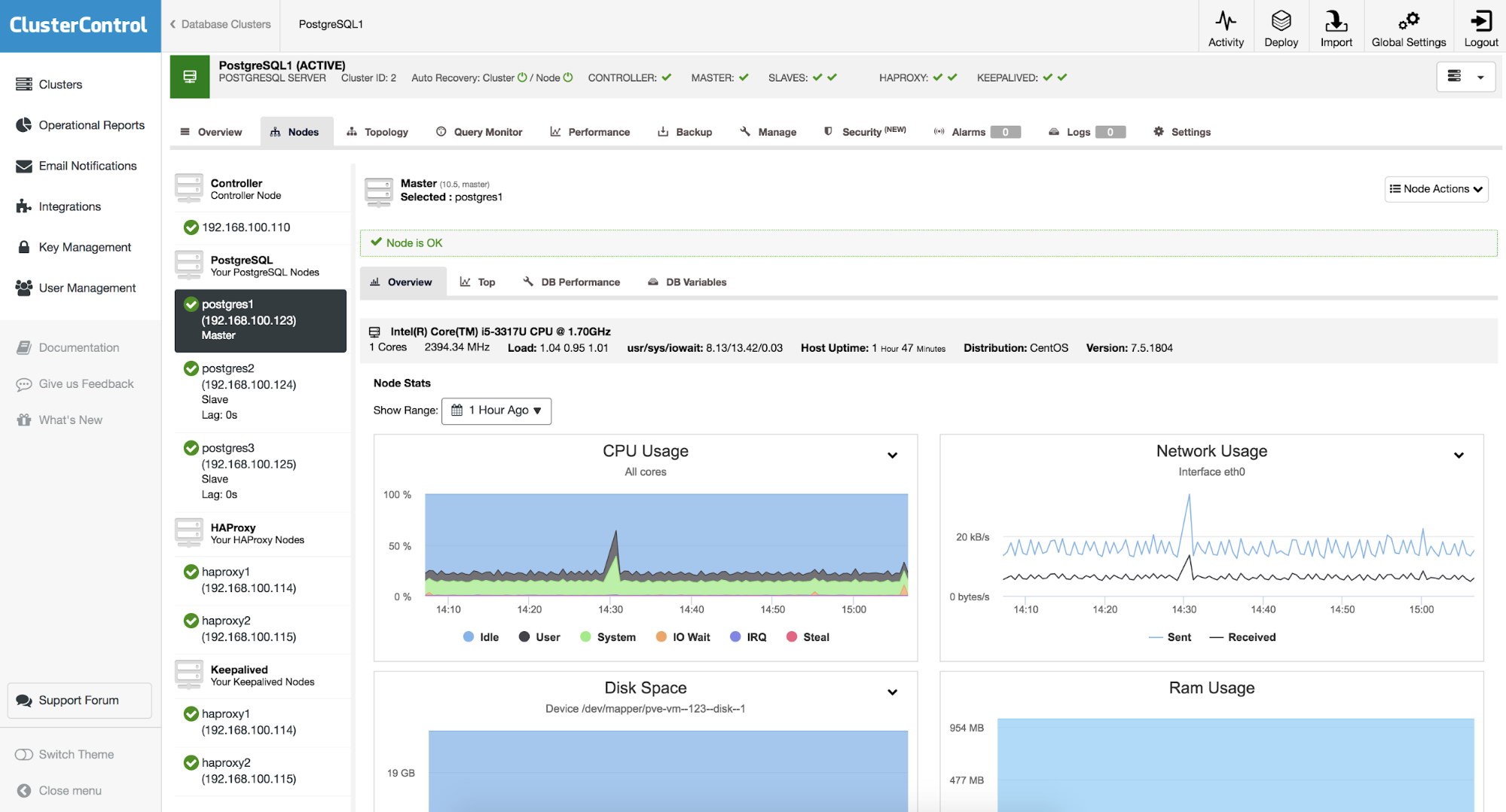
Node Overview tab
In addition to the graphs on our cluster, we can also use this functionality on each of our nodes independently. On the cluster, if we go to the “Nodes” section and select some of them, we can see an overview of it, with metrics of the operating system:
Node Overview Graphs
As we can see, we have eight graphs with information about CPU usage, Network usage, Disk space, RAM usage, Disk utilization, Disk IOPS, Swap space and Network errors, which we can use as a starting point for troubleshooting on our nodes.
ClusterControl
Single Console for Your Entire Database Infrastructure
Find out what else is new in ClusterControl
DB Performance tab
When you take a look at the node and then follow into DB Performance tab, you’ll be presented with a default of eight different metrics. You can change them or add new ones. To do that, you need to use “Choose Graph” button:
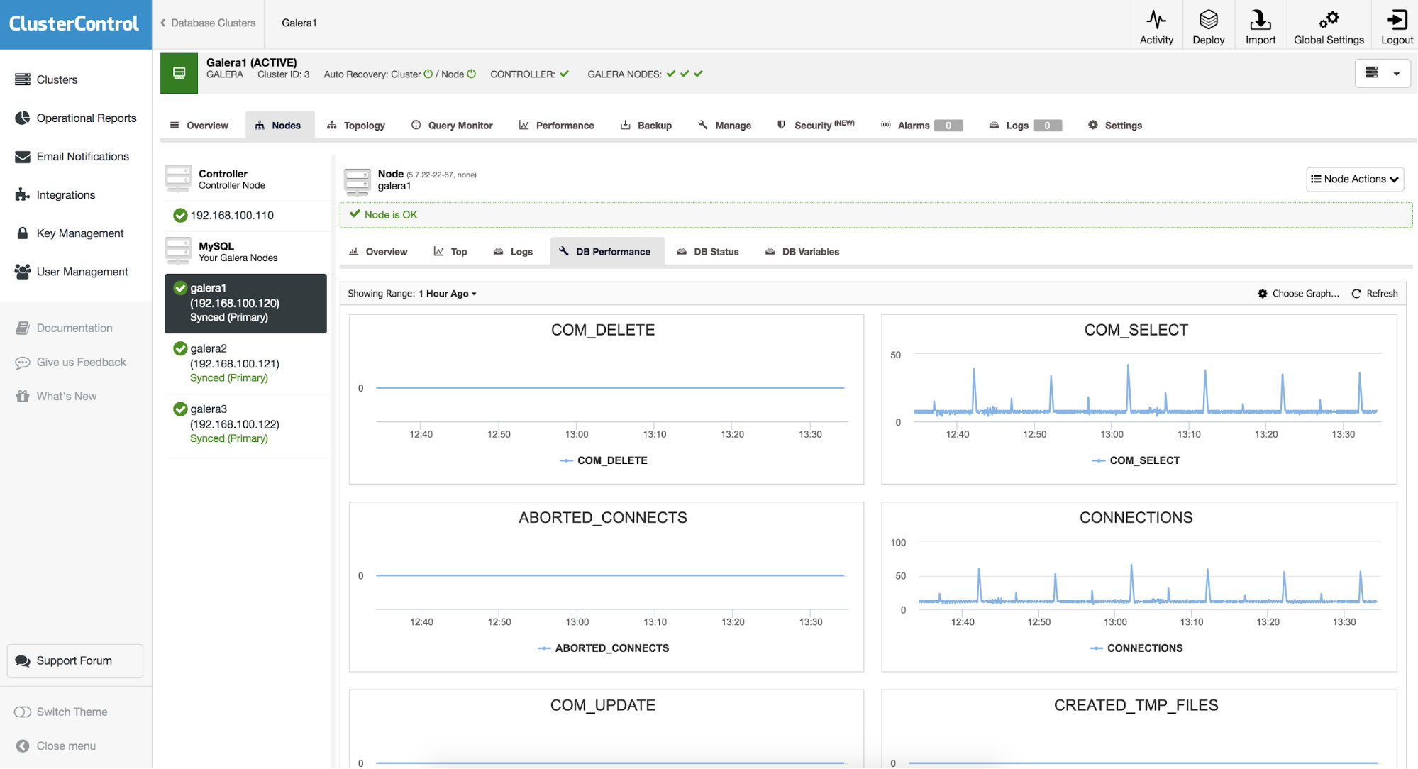
DB Performance Graphs
You’ll be presented with a new window, that allows you to configure the layout and the metrics graphed.
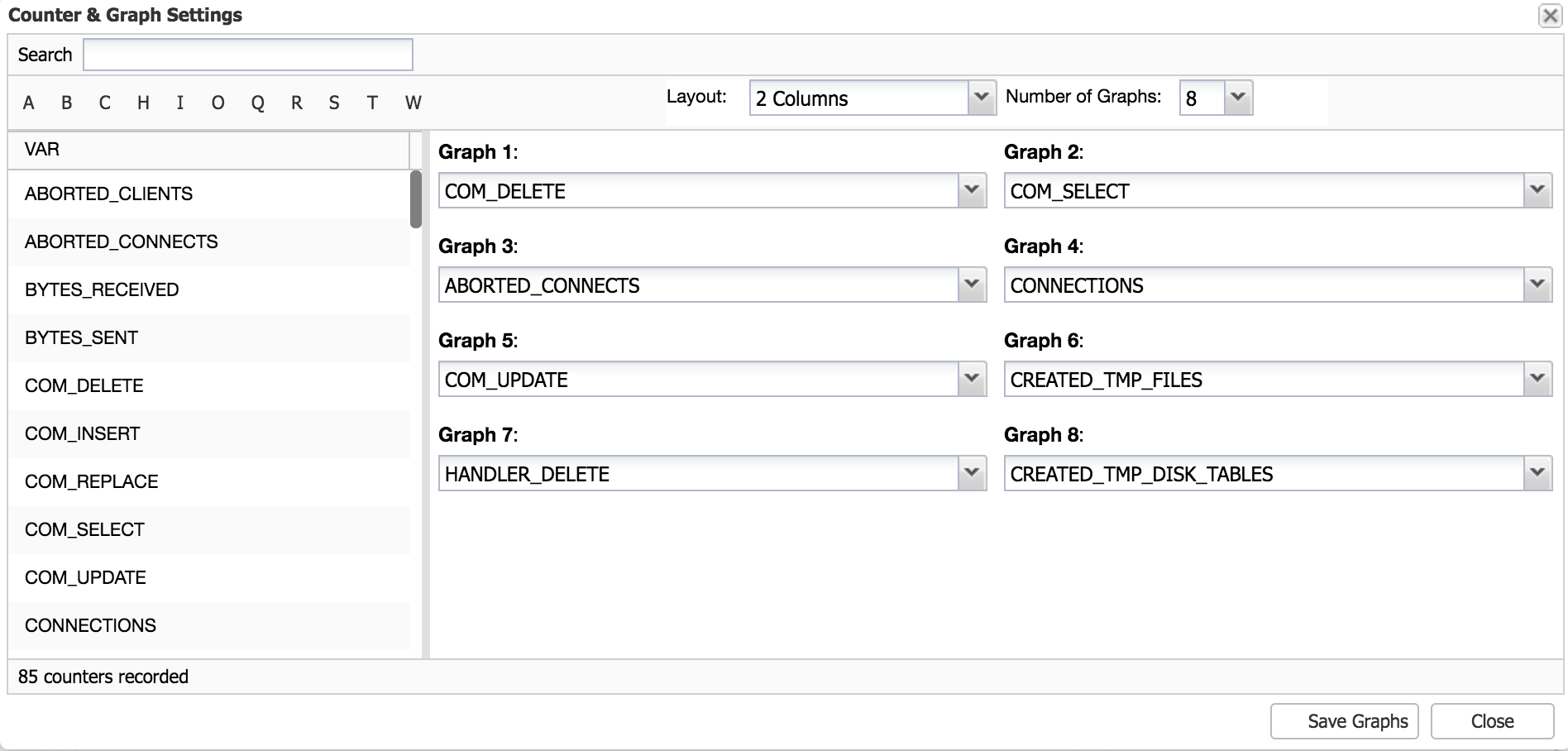
DB Performance Graphs Settings
Here you can pick the layout - two or three columns of graphs and number of graphs - up to 20. Then, you may want to modify which metrics you’d want to see plotted - use drop-down dialog boxes to pick whatever metric you’d like to add. Once you are ready, save the graphs and enjoy your new metrics.
We can also use the Operational Reports feature of ClusterControl, where we will obtain the graphs and the report of our cluster and nodes in a HTML report, that can be accessed through the ClusterControl UI, or schedule it to be sent by email periodically.
These graphs help us to have a complete picture of the state and behavior of our databases.
↧
Configuring and Managing SSL On Your MySQL Server
In this blog post, we review some of the important aspects of configuring and managing SSL in MySQL hosting. These would include the default configuration, disabling SSL, and enabling and enforcing SSL on a MySQL server. Our observations are based on the community version of MySQL 5.7.21.
Default SSL Configuration in MySQL
By default, MySQL server always installs and enables SSL configuration. However, it is not enforced that clients connect using SSL. Clients can choose to connect with or without SSL as the server allows both types of connections. Let’s see how to verify this default behavior of MySQL server.
When SSL is installed and enabled on MySQL server by default, we will typically see the following:
- Presence of *.pem files in the MySQL data directory. These are the various client and server certificates and keys that are in use for SSL as described here.
- There will be a note in the mysqld error log file during the server start, such as:
- [Note] Found ca.pem, server-cert.pem and server-key.pem in data directory. Trying to enable SSL support using them.
- Value of ‘have_ssl’ variable will be YES:
mysql> show variables like ‘have_ssl’;
+—————+——-+
| Variable_name | Value |
+—————+——-+
| have_ssl | YES |
+—————+——-+
With respect to MySQL client, by default, it always tries to go for encrypted network connection with the server, and if that fails, it falls back to unencrypted mode.
So, by connecting to MySQL server using the command:
mysql -h <hostname> -u <username> -p
We can check whether the current client connection is encrypted or not using the status command:
mysql> status
————–
mysql Ver 14.14 Distrib 5.7.21, for Linux (x86_64) using EditLine wrapper
Connection id: 75
Current database:
Current user: root@127.0.0.1
SSL: Cipher in use is DHE-RSA-AES256-SHA
Current pager: stdout
Using outfile: ”
Using delimiter: ;
Server version: 5.7.21-log MySQL Community Server (GPL)
Protocol version: 10
Connection: 127.0.0.1 via TCP/IP
…………………………..
The SSL field highlighted above indicates that the connection is encrypted. We can, however, ask the MySQL client to connect without SSL by using the command:
mysql -h <hostname> -u <username> -p –ssl-mode=DISABLED
mysql> status
————–
Connection id: 93
Current database:
Current user: sgroot@127.0.0.1
SSL: Not in use
Current pager: stdout
Using outfile: ”
Using delimiter: ;
Server version: 5.7.21-log MySQL Community Server (GPL)
Protocol version: 10
Connection: 127.0.0.1 via TCP/IP
……………………………
We can see that even though SSL is enabled on the server, we are able to connect to it without SSL.
How To Configure and Manage SSL on Your #MySQL ServerClick To Tweet
Disabling SSL in MySQL
If your requirement is to completely turn off SSL on MySQL server instead of the default option of ‘enabled, but optional mode’, we can do the following:
- Delete the *.pem certificate and key files in the MySQL data directory.
- Start MySQL with SSL option turned off. This can be done by adding a line entry:
ssl=0 in the my.cnf file.
We can observe that:
- There will NOT be any note in mysqld logs such as :
- [Note] Found ca.pem, server-cert.pem and server-key.pem in data directory. Trying to enable SSL support using them.
- Value of ‘have_ssl’ variable will be DISABLED:
mysql> show variables like ‘have_ssl’;
+—————+——-+
| Variable_name | Value |
+—————+——-+
| have_ssl | DISABLED |
+—————+——-+
Enforcing SSL in MySQL
We saw that though SSL was enabled by default on MySQL server, it was not enforced and we were still able to connect without SSL.
Now, by setting the require_secure_transport system variable, we will be able to enforce that server will accept only SSL connections. This can be verified by trying to connect to MySQL server with the command:
mysql -h <hostname> -u sgroot -p –ssl-mode=DISABLED
And, we can see that the connection would be refused with following error message from the server:
ERROR 3159 (HY000): Connections using insecure transport are prohibited while –require_secure_transport=ON.
SSL Considerations for Replication Channels
By default, in a MySQL replication setup, the slaves connect to the master without encryption.
Hence to connect to a master in a secure way for replication traffic, slaves must use MASTER_SSL=1; as part of the ‘CHANGE MASTER TO’ command which specifies parameters for connecting to the master. Please note that this option is also mandatory in case your master is configured to enforce SSL connection using require_secure_transport.

↧
[Solved] How to install MySQL Server on CentOS 7?
Recently, when I am working on setting up MySQL Enterprise Server, I found, there is too much information available over internet and it was very difficult for a newbie to get what is needed for direct implementation. So, I decided to write a quick reference guide for setting up the server, covering end to end, starting from planning to production to maintenance. This is a first post in that direction, in this post, we will discuss about installing MySQL Enterprise Server on CentOS 7 machine. Note that, the steps are same for both the Enterprise and Community editions, only binary files are different, and downloaded from different repositories.
If you are looking for installing MySQL on Windows operating system, please visit this page https://www.rathishkumar.in/2016/01/how-to-install-mysql-server-on-windows.html. I am assuming, hardware and the Operating System is installed and configured as per the requirement. Let us begin with the installation.
Removing MariaDB:
The CentOS comes with MariaDB as a default database, if you try to install, MySQL on top of it, you will encounter an error message stating the MySQL library files conflict with MariaDB library files. Remove the MariaDB to avoid errors and to have a clean installation. Use below statements to remove MariaDB completely:
sudoyum remove MariaDB-server
sudoyum remove MariaDB-client (This can be done in single step)
sudorm –rf /var/lib/mysql
sudorm /etc/my.cnf
(Run with sudo, if you are not logged in as Super Admin).
Downloading RPM files:
MySQL installation files (On CentOS 7 – rpm packages) can be downloaded from MySQL yum repository.
For MySQL Community Edition – there is clear and step-by-step guide available at the MySQL website - https://dev.mysql.com/doc/mysql-yum-repo-quick-guide/en/. The only step missing is downloading MySQL yum repository to your local machine. (This might looks very simple step, but most of the newbies, it is very helpful).
For MySQL Enterprise Edition – the binary files can be downloaded from Oracle Software Delivery Cloud (http://edelivery.oracle.com) for latest version or previous versions visit My Oracle Support (https://support.oracle.com/).
As mentioned earlier, there is a clear and step-by-step guide available at the MySQL website for Community Edition, I will be continue with installing Enterprise Edition, steps are almost same.
Choosing the RPM file:
For MySQL Community Edition, all the RPM files will be included in the downloaded YUM repository, but for Enterprise Editions, these files will be downloaded separately. (For system administration purpose, all these files can be created under a MySQL repository).
For newbies, it may be confusing to understand, the different RPM files and its contents, I am concentrating on only files required for stand-alone MySQL instances. If there is requirement for embedded MySQL or if you working on developing plugins for MySQL, can install other files. It is completely depends on your requirement. The following tables, describe the required files and where to install.
RPM File
| Description
| Location
|
mysql-commercial-server-5.7.23-1.1.el7.x86_64.rpm
|
MySQL Server and related utilities to run and administer a MySQL server.
|
On Server
|
mysql-commercial-client-5.7.23-1.1.el7.x86_64.rpm
|
Standard MySQL clients and administration tools.
|
On Server & On Client
|
mysql-commercial-common-5.7.23-1.1.el7.x86_64.rpm
|
Common files needed by MySQL client library, MySQL database server, and MySQL embedded server.
|
On Server
|
mysql-commercial-libs-5.7.23-1.1.el7.x86_64.rpm | Shared libraries for MySQL Client applications | On Server |
Installing MySQL:
Install the MySQL binary files in the following order, this is to avoid dependency errors, the following statements will install MySQL on local machine:
sudo yum localinstall mysql-commercial-libs-5.7.23-1.1.el7.x86_64.rpm
sudo yum localinstall mysql-commercial-client-5.7.23-1.1.el7.x86_64.rpm
sudo yum localinstall mysql-commercial-common-5.7.23-1.1.el7.x86_64.rpm
sudo yum localinstall mysql-commercial-server-5.7.23-1.1.el7.x86_64.rpm
Starting the MySQL Service:
On CentOS 7, the mysql service can be started by following:
sudosystemctl start mysqld.service
sudosystemctl status mysqld.service
Login to MySQL Server for first time:
Once the service is started, the superuser account ‘root’@’localhost’ created and temporary password is stored at the error log file (default /var/log/mysqld.log). The password can be retrieved by using the following command:
sudo grep 'temporary password' /var/log/mysqld.log
As soon as logged in to MySQL with the temporary password, need to reset the root password, until that, you cannot run any queries on MySQL server. You can reset the root account password by running below command.
mysql –u root –h localhost -p
alter user 'root'@'localhost' identified by 'NewPassword';
You can verify the MySQL status and edition by running the following commands, sample output provided below for MySQL 8.0 Community Edition (GPL License) running on Windows machine.
 |
| MySQL License Status |
Notes:
MySQL conflicts with MariaDB: in case if there is conflict with MariaDB, you will see the error message as below:
file /usr/share/mysql/xxx from install ofMySQL-server-xxx conflicts with file from package mariadb-libs-xxx
To resolve this error remove mariadb server and its related files from CentOS server. Refer the section - Removing mariadb.
Can’t connect to mysql server: MySQL server is installed but unable to connect from client.
Check this page for possible causes and solutions: https://www.rathishkumar.in/2017/08/solved-cannot-connect-to-mysql-server.html
Please let me know, if you are facing any other errors on comment section. i hope this post is
↧
↧
Percona XtraDB Cluster 5.6.41-28.28 Is Now Available

 Percona announces the release of Percona XtraDB Cluster 5.6.41-28.28 (PXC) on September 18, 2018. Binaries are available from the downloads section or our software repositories.
Percona XtraDB Cluster 5.6.41-28.28 is now the current release, based on the following:
- Percona Server for MySQL 5.6.41
- Codership WSREP API Rrelease 5.6.41
- Codership Galera library 3.24
Fixed Bugs
- PXC-1017: Memcached API is now disabled if node is acting as a cluster node, because InnoDB Memcached access is not replicated by Galera.
- PXC-2164: SST script compatibility with SELinux was improved by forcing it to look for port associated with the said process only.
- PXC-2155: Temporary folders created during SST execution are now deleted on cleanup.
-
PXC-2199: TOI replication protocol was fixed to prevent unexpected GTID generation caused by the
DROP TRIGGER IF EXISTSstatement logged by MySQL as a successful one due to itsIF EXISTSclause.
Help us improve our software quality by reporting any bugs you encounter using our bug tracking system. As always, thanks for your continued support of Percona!
The post Percona XtraDB Cluster 5.6.41-28.28 Is Now Available appeared first on Percona Database Performance Blog.
↧
Bloom filter and cuckoo filter
The multi-level cuckoo filter (MLCF) in SlimDB builds on the cuckoo filter (CF) so I read the cuckoo filter paper. The big deal about the cuckoo filter is that it supports delete and a bloom filter does not. As far as I know the MLCF is updated when sorted runs arrive and depart a level -- so delete is required. A bloom filter in an LSM is per sorted run and delete is not required because the filter is created when the sorted run is written and dropped when the sorted run is unlinked.
I learned of the blocked bloom filter from the cuckoo filter paper (see here or here). RocksDB uses this but I didn't know it had a name. The benefit of it is to reduce the number of cache misses per probe. I was curious about the cost and while the math is complicated, the paper estimates a 10% increase on the false positive rate for a bloom filter with 8 bits/key and a 512-bit block which is similar to a typical setup for RocksDB.
Space Efficiency
I am always interested in things that use less space for filters and block indexes with an LSM so I spent time reading the paper. It is a great paper and I hope that more people read it. The cuckoo filter (CF) paper claims better space-efficiency than a bloom filter and the claim is repeated in the SlimDB paper as:
The paper has a lot of interesting math that I was able to follow. It provides formulas for the number of bits/key for a bloom filter, cuckoo filter and semisorted cuckoo filter. The semisorted filter uses 1 less bit/key than a regular cuckoo filter. The formulas assuming E is the target false positive rate, b=4, and A is the load factor:
The target load factor is 0.95 (A = 0.95) and that comes at a cost in CPU overhead when creating the CF. Assuming A=0.95 then a bloom filter uses 10 bits/key, a cuckoo filter uses 10.53 and a semisorted cuckoo filter uses 9.47. So the cuckoo filter uses either 5% more or 5% less space than a bloom filter when the target FPR is 1% which is a different perspective from the quote I listed above. Perhaps my math is wrong and I am happy for an astute reader to explain that.
When the target FPR rate is 0.1% then a bloom filter uses 15 bits/key, a cuckoo filter uses 13.7 and a semisorted cuckoo filter uses 12.7. The savings from a cuckoo filter are larger here but the common configuration for a bloom filter in an LSM has been to target a 1% FPR. I won't claim that we have proven that FPR=1% is the best rate and recent research on Monkey has shown that we can do better when allocating space to bloom filters.
The first graph shows the number of bits/key as a function of the FPR for a bloom filter (BF) and cuckoo filter (CF). The second graph shows the ratio for bits/key from BF versus bits/key from CF. The results for semisorted CF, which uses 1 less bit/key, are not included. For the second graph a CF uses less space than a BF when the value is greater than one. The graph covers FPR from 0.00001 to 0.09 which is 0.001% to 9%. R code to generate the graphs is here.
![]()
![]()
CPU Efficiency
From the paper there is more detail on CPU efficiency in table 3, figure 5 and figure 7. Table 3 has the speed to create a filter, but the filter is much larger (192MB) than a typical per-run filter with an LSM and there will be more memory system stalls in that case. Regardless the blocked bloom filter has the least CPU overhead during construction.
Figure 5 shows the lookup performance as a function of the hit rate. Fortunately performance doesn't vary much with the hit rate. The cuckoo filter is faster than the blocked bloom filter and the block bloom filter is faster than the semisorted cuckoo filter.
Figure 7 shows the insert performance as a function of the cuckoo filter load factor. The CPU overhead per insert grows significantly when the load factor exceeds 80%.
I learned of the blocked bloom filter from the cuckoo filter paper (see here or here). RocksDB uses this but I didn't know it had a name. The benefit of it is to reduce the number of cache misses per probe. I was curious about the cost and while the math is complicated, the paper estimates a 10% increase on the false positive rate for a bloom filter with 8 bits/key and a 512-bit block which is similar to a typical setup for RocksDB.
Space Efficiency
I am always interested in things that use less space for filters and block indexes with an LSM so I spent time reading the paper. It is a great paper and I hope that more people read it. The cuckoo filter (CF) paper claims better space-efficiency than a bloom filter and the claim is repeated in the SlimDB paper as:
However, by selecting an appropriate fingerprint size f and bucket size b, it can be shown that the cuckoo filter is more space-efficient than the Bloom filter when the target false positive rate is smaller than 3%The tl;dr for me is that the space savings from a cuckoo filter is significant when the false positive rate (FPR) is sufficiently small. But when the target FPR is 1% then a cuckoo filter uses about the same amount of space as a bloom filter.
The paper has a lot of interesting math that I was able to follow. It provides formulas for the number of bits/key for a bloom filter, cuckoo filter and semisorted cuckoo filter. The semisorted filter uses 1 less bit/key than a regular cuckoo filter. The formulas assuming E is the target false positive rate, b=4, and A is the load factor:
- bloom filter: ceil(1.44 * log2(1/E))
- cuckoo filter: ceil(log2(1/E) + log2(2b)) / A == (log2(1/E) + 3) / A
- semisorted cuckoo filter: ceil(log2(1/E) + 2) / A
The target load factor is 0.95 (A = 0.95) and that comes at a cost in CPU overhead when creating the CF. Assuming A=0.95 then a bloom filter uses 10 bits/key, a cuckoo filter uses 10.53 and a semisorted cuckoo filter uses 9.47. So the cuckoo filter uses either 5% more or 5% less space than a bloom filter when the target FPR is 1% which is a different perspective from the quote I listed above. Perhaps my math is wrong and I am happy for an astute reader to explain that.
When the target FPR rate is 0.1% then a bloom filter uses 15 bits/key, a cuckoo filter uses 13.7 and a semisorted cuckoo filter uses 12.7. The savings from a cuckoo filter are larger here but the common configuration for a bloom filter in an LSM has been to target a 1% FPR. I won't claim that we have proven that FPR=1% is the best rate and recent research on Monkey has shown that we can do better when allocating space to bloom filters.
The first graph shows the number of bits/key as a function of the FPR for a bloom filter (BF) and cuckoo filter (CF). The second graph shows the ratio for bits/key from BF versus bits/key from CF. The results for semisorted CF, which uses 1 less bit/key, are not included. For the second graph a CF uses less space than a BF when the value is greater than one. The graph covers FPR from 0.00001 to 0.09 which is 0.001% to 9%. R code to generate the graphs is here.


CPU Efficiency
From the paper there is more detail on CPU efficiency in table 3, figure 5 and figure 7. Table 3 has the speed to create a filter, but the filter is much larger (192MB) than a typical per-run filter with an LSM and there will be more memory system stalls in that case. Regardless the blocked bloom filter has the least CPU overhead during construction.
Figure 5 shows the lookup performance as a function of the hit rate. Fortunately performance doesn't vary much with the hit rate. The cuckoo filter is faster than the blocked bloom filter and the block bloom filter is faster than the semisorted cuckoo filter.
Figure 7 shows the insert performance as a function of the cuckoo filter load factor. The CPU overhead per insert grows significantly when the load factor exceeds 80%.
↧
MySQL: size of your tables – tricks and tips
Many of you already know how to retrieve the size of your dataset, schemas and tables in MySQL.
To summarize, below are the different queries you can run:
Dataset Size
I the past I was using something like this :

But now with sys schema being installed by default, I encourage you to use some of the formatting functions provided with it. The query to calculate the dataset is now:
SELECT sys.format_bytes(sum(data_length)) DATA,
       sys.format_bytes(sum(index_length)) INDEXES,
       sys.format_bytes(sum(data_length + index_length)) 'TOTAL SIZE'
FROM information_schema.TABLES ORDER  BY data_length + index_length;
Let’s see an example:
Engines Used and Size
For a list of all engines used:
SELECT count(*) as '# TABLES', sys.format_bytes(sum(data_length)) DATA,
       sys.format_bytes(sum(index_length)) INDEXES,
       sys.format_bytes(sum(data_length + index_length)) 'TOTAL SIZE',
       engine `ENGINE` FROM information_schema.TABLES
WHERE TABLE_SCHEMA NOT IN ('sys','mysql', 'information_schema',
                'performance_schema', 'mysql_innodb_cluster_metadata')
GROUP BY engine;
Let’s see an example on the same database as above:

and on 5.7 with one MyISAM table (eeek):

Schemas Size
Now let’s find out which schemas are the larges:
SELECT TABLE_SCHEMA,
sys.format_bytes(sum(table_rows)) `ROWS`,
sys.format_bytes(sum(data_length)) DATA,
sys.format_bytes(sum(index_length)) IDX,
sys.format_bytes(sum(data_length) + sum(index_length)) 'TOTAL SIZE',
round(sum(index_length) / sum(data_length),2) IDXFRAC
FROM
information_schema.TABLES
GROUP By table_schema ORDER BY sum(DATA_length) DESC;

Top 10 Tables by Size
And finally a query to get the list of the 10 largest tables:
SELECT CONCAT(table_schema, '.', table_name) as 'TABLE', ENGINE,
CONCAT(ROUND(table_rows / 1000000, 2), 'M')  `ROWS`,
sys.format_bytes(data_length) DATA,
sys.format_bytes(index_length) IDX,
sys.format_bytes(data_length + index_length) 'TOTAL SIZE',
round(index_length / data_length,2) IDXFRAC
FROM   information_schema.TABLES
ORDER  BY data_length + index_length DESC LIMIT  10;

You can modify the query to retrieve the size of any given table of course.
That was the theory and it’s always good to see those queries time to time.
But…
But can we trust these results ? In fact, sometimes, this can be very tricky, let’s check this example:
mysql> SELECT COUNT(*) AS TotalTableCount ,table_schema,
CONCAT(ROUND(SUM(table_rows)/1000000,2),'M') AS TotalRowCount,
CONCAT(ROUND(SUM(data_length)/(1024*1024*1024),2),'G') AS TotalTableSize,
CONCAT(ROUND(SUM(index_length)/(1024*1024*1024),2),'G') AS TotalTableIndex,
CONCAT(ROUND(SUM(data_length+index_length)/(1024*1024*1024),2),'G') TotalSize
FROM information_schema.TABLES GROUP BY table_schema
ORDER BY SUM(data_length+index_length)  DESC LIMIT 1;
+-----------------+--------------+---------------+----------------+-----------------+-----------+
| TotalTableCount | TABLE_SCHEMA | TotalRowCount | TotalTableSize | TotalTableIndex | TotalSize |
+-----------------+--------------+---------------+----------------+-----------------+-----------+
|              15 | wp_lefred    | 0.02M         | 5.41G          | 0.00G           | 5.41G     |
+-----------------+--------------+---------------+----------------+-----------------+-----------+
This seems to be a very large table ! Let’s verify this:
mysql> select * from information_schema.TABLES
       where table_schema='wp_lefred' and table_name = 'wp_options'\G
*************************** 1. row ***************************
  TABLE_CATALOG: def
   TABLE_SCHEMA: wp_lefred
     TABLE_NAME: wp_options
     TABLE_TYPE: BASE TABLE
         ENGINE: InnoDB
        VERSION: 10
     ROW_FORMAT: Dynamic
     TABLE_ROWS: 3398
 AVG_ROW_LENGTH: 1701997
    DATA_LENGTH: 5783388160
MAX_DATA_LENGTH: 0
   INDEX_LENGTH: 442368
      DATA_FREE: 5242880
 AUTO_INCREMENT: 1763952
    CREATE_TIME: 2018-09-18 00:29:16
    UPDATE_TIME: 2018-09-17 23:44:40
     CHECK_TIME: NULL
TABLE_COLLATION: utf8mb4_unicode_ci
       CHECKSUM: NULL
 CREATE_OPTIONS:
  TABLE_COMMENT:
1 row in set (0.01 sec)
In fact we can see that the average row length is pretty big.
So let’s verify on the disk:
[root@vps21575 database]# ls -lh wp_lefred/wp_options.ibd
-rw-r----- 1 mysql mysql 11M Sep 18 00:31 wp_lefred/wp_options.ibd
11M ?! The table is 11M but Information_Schema thinks it’s 5.41G ! Quite a big difference !
In fact this is because InnoDB creates these statistics from a very small amount of pages by default.
So if you have a lot of records with a very variable size like it’s the case with this WordPress table, it could be safer to
increase the amount of pages used to generate those statistics:
mysql> set global innodb_stats_transient_sample_pages= 100;
Query OK, 0 rows affected (0.00 sec)

mysql> analyze table wp_lefred.wp_options;
+----------------------+---------+----------+----------+
| Table                | Op      | Msg_type | Msg_text |
+----------------------+---------+----------+----------+
| wp_lefred.wp_options | analyze | status   | OK       |
+----------------------+---------+----------+----------+
1 row in set (0.05 sec)

Let's check the table statistics now:
*************************** 1. row ***************************
  TABLE_CATALOG: def
   TABLE_SCHEMA: wp_lefred
     TABLE_NAME: wp_options
     TABLE_TYPE: BASE TABLE
         ENGINE: InnoDB
        VERSION: 10
     ROW_FORMAT: Dynamic
     TABLE_ROWS: 3075
 AVG_ROW_LENGTH: 1198
    DATA_LENGTH: 3686400
MAX_DATA_LENGTH: 0
   INDEX_LENGTH: 360448
      DATA_FREE: 4194304
 AUTO_INCREMENT: 1764098
    CREATE_TIME: 2018-09-18 00:34:07
    UPDATE_TIME: 2018-09-18 00:32:55
     CHECK_TIME: NULL
TABLE_COLLATION: utf8mb4_unicode_ci
       CHECKSUM: NULL
 CREATE_OPTIONS:
  TABLE_COMMENT:
1 row in set (0.01 sec)
We can see that the average row length is much smaller now (and could be smaller with an even bigger sample).
Let’s verify:
mysql> SELECT CONCAT(table_schema, '.', table_name) as 'TABLE', ENGINE,
    -> CONCAT(ROUND(table_rows / 1000000, 2), 'M')  `ROWS`,
    -> sys.format_bytes(data_length) DATA,
    -> sys.format_bytes(index_length) IDX,
    -> sys.format_bytes(data_length + index_length) 'TOTAL SIZE',
    -> round(index_length / data_length,2) IDXFRAC
    -> FROM   information_schema.TABLES
    -> WHERE table_schema='wp_lefred' and table_name = 'wp_options';
+----------------------+--------+-------+----------+------------+------------+---------+
| TABLE                | ENGINE | ROWS  | DATA     | IDX        | TOTAL SIZE | IDXFRAC |
+----------------------+--------+-------+----------+------------+------------+---------+
| wp_lefred.wp_options | InnoDB | 0.00M | 3.52 MiB | 352.00 KiB | 3.86 MiB   |    0.10 |
+----------------------+--------+-------+----------+------------+------------+---------+
In fact, this table uses a long text as column and it can be filled with many things or almost nothing.
We can verify that for this particular table we have some very large values:
mysql> select CHAR_LENGTH(option_value), count(*)
       from wp_lefred.wp_options group by 1 order by 1 desc limit 10;
+---------------------------+----------+
| CHAR_LENGTH(option_value) | count(*) |
+---------------------------+----------+
|                    245613 |        1 |
|                    243545 |        2 |
|                    153482 |        1 |
|                    104060 |        1 |
|                     92871 |        1 |
|                     70468 |        1 |
|                     60890 |        1 |
|                     41116 |        1 |
|                     33619 |        5 |
|                     33015 |        2 |
+---------------------------+----------+
Even if the majority of the records are much smaller:
mysql> select CHAR_LENGTH(option_value), count(*)
       from wp_lefred.wp_options group by 1 order by 2 desc limit 10;
+---------------------------+----------+
| CHAR_LENGTH(option_value) | count(*) |
+---------------------------+----------+
|                        10 |     1485 |
|                        45 |      547 |
|                        81 |      170 |
|                         6 |      167 |
|                         1 |       84 |
|                        83 |       75 |
|                        82 |       65 |
|                        84 |       60 |
|                        80 |       44 |
|                        30 |       42 |
+---------------------------+----------+
Conclusion
So in general, using Information_Schema provides a good overview of the tables size, but please always verify the size on disk to see if it matches because when a table contains records that can have a large variable size, those statistics are often incorrect because the InnoDB page sample used is too small.
But don’t forget that on disk, table spaces can also be fragmented !
↧
How to Monitor multiple MySQL instances running on the same machine - ClusterControl Tips & Tricks

Requires ClusterControl 1.6 or later. Applies to MySQL based instances/clusters.
On some occasions, you might want to run multiple instances of MySQL on a single machine. You might want to give different users access to their own MySQL servers that they manage themselves, or you might want to test a new MySQL release while keeping an existing production setup undisturbed.
It is possible to use a different MySQL server binary per instance, or use the same binary for multiple instances (or a combination of the two approaches). For example, you might run a server from MySQL 5.6 and one from MySQL 5.7, to see how the different versions handle a certain workload. Or you might run multiple instances of the latest MySQL version, each managing a different set of databases.
Whether or not you use distinct server binaries, each instance that you run must be configured with unique values for several operating parameters. This eliminates the potential for conflict between instances. You can use MySQL Sandbox to create multiple MySQL instances. Or you can use mysqld_multi available in MySQL to start or stop any number of separate mysqld processes running on different TCP/IP ports and UNIX sockets.
In this blog post, we’ll show you how to configure ClusterControl to monitor multiple MySQL instances running on one host.
ClusterControl Limitation
At the time of writing, ClusterControl does not support monitoring of multiple instances on one host per cluster/server group. It assumes the following best practices:
- Only one MySQL instance per host (physical server or virtual machine).
- MySQL data redundancy should be configured on N+1 server.
- All MySQL instances are running with uniform configuration across the cluster/server group, e.g., listening port, error log, datadir, basedir, socket are identical.
With regards to the points mentioned above, ClusterControl assumes that in a cluster/server group:
- MySQL instances are configured uniformly across a cluster; same port, the same location of logs, base/data directory and other critical configurations.
- It monitors, manages and deploys only one MySQL instance per host.
- MySQL client must be installed on the host and available on the executable path for the corresponding OS user.
- The MySQL is bound to an IP address reachable by ClusterControl node.
- It keeps monitoring the host statistics e.g CPU/RAM/disk/network for each MySQL instance individually. In an environment with multiple instances per host, you should expect redundant host statistics since it monitors the same host multiple times.
With the above assumptions, the following ClusterControl features do not work for a host with multiple instances:
Backup - Percona Xtrabackup does not support multiple instances per host and mysqldump executed by ClusterControl only connects to the default socket.
Process management - ClusterControl uses the standard ‘pgrep -f mysqld_safe’ to check if MySQL is running on that host. With multiple MySQL instances, this is a false positive approach. As such, automatic recovery for node/cluster won’t work.
Configuration management - ClusterControl provisions the standard MySQL configuration directory. It usually resides under /etc/ and /etc/mysql.
Workaround
Monitoring multiple MySQL instances on a machine is still possible with ClusterControl with a simple workaround. Each MySQL instance must be treated as a single entity per server group.
In this example, we have 3 MySQL instances on a single host created with MySQL Sandbox:

ClusterControl monitoring multiple instances on same host
We created our MySQL instances using the following commands:
$ su - sandbox
$ make_multiple_sandbox mysql-5.7.23-linux-glibc2.12-x86_64.tar.gz
By default, MySQL Sandbox creates mysql instances that listen to 127.0.0.1. It is necessary to configure each node appropriately to make them listen to all available IP addresses. Here is the summary of our MySQL instances in the host:
[sandbox@master multi_msb_mysql-5_7_23]$ cat default_connection.json
{
"node1":
    {
        "host":     "master",
        "port":     "15024",
        "socket":   "/tmp/mysql_sandbox15024.sock",
        "username": "msandbox@127.%",
        "password": "msandbox"
    }
,
"node2":
    {
        "host":     "master",
        "port":     "15025",
        "socket":   "/tmp/mysql_sandbox15025.sock",
        "username": "msandbox@127.%",
        "password": "msandbox"
    }
,
"node3":
    {
        "host":     "master",
        "port":     "15026",
        "socket":   "/tmp/mysql_sandbox15026.sock",
        "username": "msandbox@127.%",
        "password": "msandbox"
    }
}
Next step is to modify the configuration of the newly created instances. Go to my.cnf for each of them and hash bind_address variable:
[sandbox@master multi_msb_mysql-5_7_23]$ ps -ef | grep mysqld_safe
sandbox  13086     1  0 08:58 pts/0    00:00:00 /bin/sh bin/mysqld_safe --defaults-file=/home/sandbox/sandboxes/multi_msb_mysql-5_7_23/node1/my.sandbox.cnf
sandbox  13805     1  0 08:58 pts/0    00:00:00 /bin/sh bin/mysqld_safe --defaults-file=/home/sandbox/sandboxes/multi_msb_mysql-5_7_23/node2/my.sandbox.cnf
sandbox  14065     1  0 08:58 pts/0    00:00:00 /bin/sh bin/mysqld_safe --defaults-file=/home/sandbox/sandboxes/multi_msb_mysql-5_7_23/node3/my.sandbox.cnf
[sandbox@master multi_msb_mysql-5_7_23]$ vi my.cnf
#bind_address = 127.0.0.1
Then install mysql on your master node and restart all instances using restart_all script.
[sandbox@master multi_msb_mysql-5_7_23]$ yum install mysql
[sandbox@master multi_msb_mysql-5_7_23]$ ./restart_all
# executing "stop" on /home/sandbox/sandboxes/multi_msb_mysql-5_7_23
executing "stop" on node 1
executing "stop" on node 2
executing "stop" on node 3
# executing "start" on /home/sandbox/sandboxes/multi_msb_mysql-5_7_23
executing "start" on node 1
. sandbox server started
executing "start" on node 2
. sandbox server started
executing "start" on node 3
. sandbox server started
From ClusterControl, we need to perform ‘Import’ for each instance as we need to isolate them in a different group to make it work.

ClusterControl import existing server
For node1, enter the following information in ClusterControl > Import:

ClusterControl import existing server
Make sure to put proper ports (different for different instances) and host (same for all instances).
You can monitor the progress by clicking on the Activity/Jobs icon in the top menu.

ClusterControl import existing server details
You will see node1 in the UI once ClusterControl finishes the job. Repeat the same steps to add another two nodes with port 15025 and 15026. You should see something like the below once they are added:

ClusterControl Dashboard
There you go. We just added our existing MySQL instances into ClusterControl for monitoring. Happy monitoring!
PS.: To get started with ClusterControl, click here!
↧
↧
sysbench for MySQL 8.0

Alexey made this amazing tool that the majority of MySQL DBAs are using, but if you use sysbench provided with your GNU/Linux distribution or its repository on packagecloud.io you won’t be able to use it with the new default authentication plugin in MySQL 8.0 (caching_sha2_password).
This is because most of the sysbench binaries are compiled with the MySQL 5.7 client library or MariaDB ones. There is an issue on github where Alexey explains this.
So if you want to use sysbench with MySQL 8.0 and avoid the message below,
error 2059: Authentication plugin 'caching_sha2_password' cannot be loaded:
/usr/lib64/mysql/plugin/caching_sha2_password.so: cannot open shared object file:
No such file or directory
you have 3 options:
- modify the use to use
mysql_native_passwordas authentication method - compile sysbench linking it to
mysql-community-libs-8.0.x(/usr/lib64/mysql/libmysqlclient.so.21) - use the rpm for RHEL7/CentOS7/OL7 available on this post:
↧
Durability debt
I define durability debt to be the amount of work that can be done to persist changes that have been applied to a database. Dirty pages must be written back for a b-tree. Compaction must be done for an LSM. Durability debt has IO and CPU components. The common IO overhead is from writing something back to the database. The common CPU overhead is from computing a checksum and optionally from compressing data.
From an incremental perspective (pending work per modified row) an LSM usually has less IO and more CPU durability debt than a B-Tree. From an absolute perspective the maximum durability debt can be much larger for an LSM than a B-Tree which is one reason why tuning can be more challenging for an LSM than a B-Tree.
In this post by LSM I mean LSM with leveled compaction.
B-Tree
The maximum durability debt for a B-Tree is limited by the size of the buffer pool. If the buffer pool has N pages then there will be at most N dirty pages to write back. If the buffer pool is 100G then there will be at most 100G to write back. The IO is more random or less random depending on whether the B-Tree is update-in-place, copy-on-write random or copy-on-write sequential. I prefer to describe this as small writes (page at a time) or large writes (many pages grouped into a larger block) rather than random or sequential. InnoDB uses small writes and WiredTiger uses larger writes. The distinction between small writes and large writes is more important with disks than with SSD.
There is a small CPU overhead from computing the per-page checksum prior to write back. There can be a larger CPU overhead from compressing the page. Compression isn't popular with InnoDB but is popular with WiredTiger.
There can be an additional IO overhead when torn-write protection is enabled as provided by the InnoDB double write buffer.
LSM
The durability debt for an LSM is the work required to compact all data into the max level (Lmax). A byte in the write buffer causes more debt than a byte in the L1 because more work is needed to move the byte from the write buffer to Lmax than from L1 to Lmax.
The maximum durability debt for an LSM is limited by the size of the storage device. Users can configure RocksDB such that the level 0 (L0) is huge. Assume that the database needs 1T of storage were it compacted into one sorted run and the write-amplification to move data from the L0 to the max level (Lmax) is 30. Then the maximum durability debt is 30 * sizeof(L0). The L0 is usually configured to be <= 1G in which case the durability debt from the L0 is <= 30G. But were the L0 configured to be <= 1T then the debt from it could grow to 30T.
I use the notion of per-level write-amp to explain durability debt in an LSM. Per-level write-amp is defined in the next section. Per-level write-amp is a proxy for all of the work done by compaction, not just the data to be written. When the per-level write-amp is X then for compaction from Ln to Ln+1 for every key-value pair from Ln there are ~X key-value pairs from Ln+1 for which work is done including:
Per-level write-amp in an LSM
The per-level write-amplification is the work required to move data between adjacent levels. The per-level write-amp for the write buffer is 1 because a write buffer flush creates a new SST in L0 without reading/re-writing an SST already in L0.
I assume that any key in Ln is already in Ln+1 so that merging Ln into Ln+1 does not make Ln+1 larger. This isn't true in real life, but this is a model.
The per-level write-amp for Ln is approximately sizeof(Ln+1) / sizeof(Ln). For n=0 this is 2 with a typical RocksDB configuration. For n>0 this is the per-level growth factor and the default is 10 in RocksDB. Assume that the per-level growth factor is equal to X, in reality the per-level write-amp is f*X rather than X where f ~= 0.7. See this excellent paper or examine the compaction IO stats from a production RocksDB instance. Too many excellent conference papers assume it is X rather than f*X in practice.
The per-level write-amp for Lmax is 0 because compaction stops at Lmax.
From an incremental perspective (pending work per modified row) an LSM usually has less IO and more CPU durability debt than a B-Tree. From an absolute perspective the maximum durability debt can be much larger for an LSM than a B-Tree which is one reason why tuning can be more challenging for an LSM than a B-Tree.
In this post by LSM I mean LSM with leveled compaction.
B-Tree
The maximum durability debt for a B-Tree is limited by the size of the buffer pool. If the buffer pool has N pages then there will be at most N dirty pages to write back. If the buffer pool is 100G then there will be at most 100G to write back. The IO is more random or less random depending on whether the B-Tree is update-in-place, copy-on-write random or copy-on-write sequential. I prefer to describe this as small writes (page at a time) or large writes (many pages grouped into a larger block) rather than random or sequential. InnoDB uses small writes and WiredTiger uses larger writes. The distinction between small writes and large writes is more important with disks than with SSD.
There is a small CPU overhead from computing the per-page checksum prior to write back. There can be a larger CPU overhead from compressing the page. Compression isn't popular with InnoDB but is popular with WiredTiger.
There can be an additional IO overhead when torn-write protection is enabled as provided by the InnoDB double write buffer.
LSM
The durability debt for an LSM is the work required to compact all data into the max level (Lmax). A byte in the write buffer causes more debt than a byte in the L1 because more work is needed to move the byte from the write buffer to Lmax than from L1 to Lmax.
The maximum durability debt for an LSM is limited by the size of the storage device. Users can configure RocksDB such that the level 0 (L0) is huge. Assume that the database needs 1T of storage were it compacted into one sorted run and the write-amplification to move data from the L0 to the max level (Lmax) is 30. Then the maximum durability debt is 30 * sizeof(L0). The L0 is usually configured to be <= 1G in which case the durability debt from the L0 is <= 30G. But were the L0 configured to be <= 1T then the debt from it could grow to 30T.
I use the notion of per-level write-amp to explain durability debt in an LSM. Per-level write-amp is defined in the next section. Per-level write-amp is a proxy for all of the work done by compaction, not just the data to be written. When the per-level write-amp is X then for compaction from Ln to Ln+1 for every key-value pair from Ln there are ~X key-value pairs from Ln+1 for which work is done including:
- Read from Ln+1. If Ln is a small level then the data is likely to be in the LSM block cache or OS page cache. Otherwise it is read from storage. Some reads will be cached, all writes go to storage. So the write rate to storage is > the read rate from storage.
- The key-value pairs are decompressed if the level is compressed for each block not in the LSM block cache.
- The key-value pairs from Ln+1 are merged with Ln. Note that this is a merge, not a merge sort because the inputs are ordered. The number of comparisons might be less than you expect because one iterator is ~X times larger than the other and there are optimizations for that.
The output from the merge is then compressed and written back to Ln+1. Some of the work above (reads, decompression) are also done for Ln but most of the work comes from Ln+1 because it is many times larger than Ln. I stated above that an LSM usually has more IO and less CPU durability debt per modified row. The extra CPU overheads come from decompression and the merge. I am not sure whether to count the compression overhead as extra.
Assuming the per-level growth factor is 10 and f is 0.7 (see below) then the per-level write-amp is 7 for L1 and larger levels. If sizeof(L1) == sizeof(L0) then the per-level write-amp is 2 for the L0. And the per-level write-amp is always 1 for the write buffer.
From this we can estimate the pending write-amp for data at any level in the LSM tree.
- Key-value pairs in the write buffer have the most pending write-amp. Key-value pairs in the max level (L5 in this case) have none. Key-value pairs in the write buffer are further from the max level.
- Starting with the L2 there is more durability debt from a full Ln+1 than a full Ln -- while there is more pending write-amp for Ln, there is more data in Ln+1.
- Were I given the choice of L1, L2, L3 and L4 when first placing a write in the LSM tree then I would choose L4 as that has the least pending write-amp.
- Were I to choose to make one level 10% larger then I prefer to do that for a smaller level given the values in the rel size X pend column.
legend:
w-amp per-lvl : per-level write-amp
w-amp pend : write-amp to move byte to Lmax from this level
rel size : size of level relative to write buffer
rel size X pend : write-amp to move all data from that level to Lmax
w-amp w-amp rel rel size
level per-lvl pend size X pend
----- ------- ----- ----- --------
wbuf 1 31 1 31
L0 2 30 4 120
L1 7 28 4 112
L2 7 21 40 840
L3 7 14 400 5600
L4 7 7 4000 28000
L5 0 0 40000 0
Per-level write-amp in an LSM
The per-level write-amplification is the work required to move data between adjacent levels. The per-level write-amp for the write buffer is 1 because a write buffer flush creates a new SST in L0 without reading/re-writing an SST already in L0.
I assume that any key in Ln is already in Ln+1 so that merging Ln into Ln+1 does not make Ln+1 larger. This isn't true in real life, but this is a model.
The per-level write-amp for Ln is approximately sizeof(Ln+1) / sizeof(Ln). For n=0 this is 2 with a typical RocksDB configuration. For n>0 this is the per-level growth factor and the default is 10 in RocksDB. Assume that the per-level growth factor is equal to X, in reality the per-level write-amp is f*X rather than X where f ~= 0.7. See this excellent paper or examine the compaction IO stats from a production RocksDB instance. Too many excellent conference papers assume it is X rather than f*X in practice.
The per-level write-amp for Lmax is 0 because compaction stops at Lmax.
↧
Production Secret Management at Airbnb
Our philosophy and approach to production secret management

Airbnb is a global community built on trust. The Security team helps to build trust by maintaining security standards to store, manage and access sensitive information assets. These include secrets, such as API keys and database credentials. Applications use secrets to provide everyday site features, and those secrets used to access production resources are particularly important to protect. This is why we built an internal system we call Bagpiper to securely manage all production secrets.
Bagpiper is a collection of tools and framework components Airbnb uses in all aspects of production secret management. This includes storage, rotation and access. More importantly, Bagpiper provides a safe, repeatable pattern that can be applied across Engineering. It is designed to be language and environment agnostic, and supports our evolving production infrastructure. To better understand what Bagpiper is, it is worth understanding our design considerations.
Design Goals
A few years ago, the majority of Airbnb’s application configurations were managed using Chef. These configurations included secrets, which were stored in Chef encrypted databags. Chef helped us to progress towards having infrastructure as code, but led to usability problems for our engineers because applications were deployed using a separate system. As Airbnb grew, these challenges became significant opportunities to improve our operational efficiency.
To scale with Airbnb’s growth we needed to decouple secret management from Chef, so we built Bagpiper to provide strong security and operational excellence. We aimed to achieve these goals:
- Provide a least-privileged access pattern
- Allow secrets to be encrypted at rest
- Support applications across different languages and environments
- Manage secrets for periodic rotation
- Align with Airbnb’s engineering patterns
- Scale with Airbnb’s evolving infrastructure
Segmentation and Access-Control
Bagpiper creates segmented access by asymmetrically encrypting secrets with service-specific keys. At Airbnb, services are created with basic scaffolds to support common features such as inter-service communication. At this time, an unique IAM role and a public/private key-pair is also created. The private key is encrypted by AWS’ key management service (KMS) using envelope encryption. The encrypted content is tied to the service’s IAM role, so none other than the service itself can decrypt it.
Selected services access each secret through a per-secret keychain. Bagpiper encrypts a secret with each of the public keys found on the keychain. Only those services that possess the corresponding private keys can decrypt the secret. Envelope encryption is used to encrypt the secret but it is made transparent to the user. In our deployment, a production application will first invoke KMS to decrypt the private key, and then use it to decrypt any number of secrets that it is allowed to access. Since most of the operations happen offline, it is scalable and cost effective to deploy.
Encrypted at Rest and Decrypted on Use
Bagpiper allows engineers to add, remove and rotate secrets, or to make them available to selected production systems. Bagpiper translates this work to file changes and writes them to disk as databag files. Databags are JSON formatted files with similar structures as Chef encrypted databags. Databag files, along with the encrypted key files and code are checked into applications’ Git repositories.
Changes to secrets go through the same change-release process as code. This includes peer review, continuous integration (CI) and deployment. During CI, databags and key files are incorporated into application build artifacts. On deployment, applications use the Bagpiper client library to read secrets from databags. With Bagpiper, applications are able to access secrets securely. At the same time, deploying secrets together with code changes simplifies the release process. Application states from forward deployments and rollbacks are predictable and repeatable. We are able to progress towards having infrastructure as code with improved operational safety.
Application Support and Integration
Many technologies we use today did not exist at Airbnb a few years ago, and many more are yet to be built. To build for the future of Airbnb, Bagpiper must be able to support a variety of applications across different languages and environments. We achieved this goal with the Bagpiper runtime-image, a cross-platform executable that abstracts parsing and decrypting databags. It is written in Java, and then built into platform-specific runtime-images using the jlink tool. Bagpiper runtime-image runs on Linux, OSX and Windows systems without a Java runtime environment (JRE). It is installed across different application environments and found in the file systems.
Bagpiper can support different types of applications cost-effectively. Today, majority of Airbnb’s applications are written in Java and Ruby. Therefore, we created lightweight client libraries for Java and Ruby applications to securely access secrets. Underneath, these client libraries read databags and key files from the build artifact and directly invoke the Bagpiper runtime-image from the file system. Client libraries receive the secrets and make them available to the application idiomatically.
Secret Rotation on a Continual Basis
Best practice is to rotate secrets periodically. Bagpiper helps to enforce a secret rotation policy with per-secret annotated data. Secret annotations are key-value pairs that can specify when a secret was created or last rotated, and when it should be rotated again. Annotated data is encoded and stored alongside the encrypted secret inside databag files. Though it is unencrypted, it is cryptographically tied to the secret, so tampering is not possible.
Today, a small but growing number of secrets are annotated for the purpose of managed rotation. A scheduled job periodically scans application Git repositories to find secrets that are eligible to be rotated. These secrets are tracked through an internal vulnerability management system, so that application owners are held accountable. Sometimes it is possible to generate secrets, for example MySQL database credentials. If this is described in the annotations, a pull request that contains the file changes for the rotated secret is created for the application owner to review and deploy.
Putting it All Together
We looked at Bagpiper from several different angles. It is a secret management solution that uses a non-centralized, offline architecture that is different from many of the alternative products. Bagpiper leverages Airbnb’s infrastructure as much as possible and uses a Git-based change-release pattern that Airbnb is already familiar with. This approach has helped us to meet our secret management needs across different application environments. To help put everything into perspective, see an architectural diagram below:
Concluding Thoughts
A secure and repeatable secret management practice is critical to a company that is undergoing rapid growth and transformation. It also presents many unique technical challenges and tradeoffs. We hope sharing Airbnb’s philosophy and approach is helpful to those that face similar challenges. As we remain focused on building technology to protect our community, we are grateful for our leaders within Airbnb for their continued investment, commitment and support.
Want to help protect our community? The Security team is always looking for talented people to join our team!
Many thanks to Paul Youn, Jon Tai, Bruce Sherrod, Lifeng Sang and Anthony Lugo for reviewing this blog post before it was published
Production Secret Management at Airbnb was originally published in Airbnb Engineering & Data Science on Medium, where people are continuing the conversation by highlighting and responding to this story.
↧
ProxySQL 1.4.10 and Updated proxysql-admin Tool Now in the Percona Repository

 ProxySQL 1.4.10, released by ProxySQL, is now available for download in the Percona Repository along with an updated version of Percona’s proxysql-admin tool.
ProxySQL is a high-performance proxy, currently for MySQL and its forks (like Percona Server for MySQL and MariaDB). It acts as an intermediary for client requests seeking resources from the database. René Cannaò created ProxySQL for DBAs as a means of solving complex replication topology issues.
The ProxySQL 1.4.10 source and binary packages available at https://percona.com/downloads/proxysql include ProxySQL Admin – a tool, developed by Percona to configure Percona XtraDB Cluster nodes into ProxySQL. Docker images for release 1.4.10 are available as well: https://hub.docker.com/r/percona/proxysql/. You can download the original ProxySQL from https://github.com/sysown/proxysql/releases.
Improvements
- PSQLADM-12: Implemented the writer-is-reader option in proxysql-admin. This is now a text option: ‘always’, ‘never’, and ‘ondemand’
-
PSQLADM-64: Added the option
--sync-multi-cluster-userswhich , that uses the same function as--sync-usersbut will not delete users on ProxySQL that don’t exist on MySQL - PSQLADM-90: Added testsuites for host priority/slave/loadbal/writer-is-reader features
-
Additional debugging support
An additional--debugflag on scripts prints more output. All SQL calls are now logged if debugging is enabled.
Tool Enhancements
-
proxysql-status
proxysql-status now reads the credentials from theproxysql-admin.cnffile. It is possible to look only at certain tables (--files,--main,--monitor,--runtime,--stats). Also added the ability to filter based on the table name (--table) -
tests directory
Theproxysql-admin-testsuite.shscript can now be used to create test clusters (proxysql-admin-testsuite.sh <workdir> --no-test --cluster-one-only
, this option will create a 3-node PXC cluster with 1 async slave and will also start proxyxql). Also added regression test suites. -
tools directory
Added extra tools that can be used for debugging (mysql_exec,proxysql_exec,enable_scheduler, andrun_galera_checker).
Bug Fixes
-
PSQLADM-73:
proxysql-admindid not check that the monitor user had been configured on the PXC nodes. -
PSQLADM-82: the
without-check-monitor-useroption did check the monitor user (even if it was enabled). This option has been replaced withuse-existing-monitor-password. -
PSQLADM-83:
proxysql_galera-checkercould hang if there was no scheduler entry. -
PSQLADM-87: in some cases,
proxysql_galera_checkerwas not moving a node toOFFLINE_SOFTif pxc_maint_mode was set to “maintenance” -
PSQLADM-88:
proxysql_node_monitorwas searching among all nodes, not just the read hostgroup. - PSQLADM-91: Nodes in the priority list were not being picked.
- PSQLADM-93: If mode=’loadbal’, then the read_hostgroup setting was used from the config file, rather than being set to -1.
-
PSQLADM-96: Centos used
/usr/share/proxysqlrather than/var/lib/proxysql - PSQLADM-98: In some cases, checking the PXC node status could stall (this call now uses a TIMEOUT)
ProxySQL is available under OpenSource license GPLv3.
The post ProxySQL 1.4.10 and Updated proxysql-admin Tool Now in the Percona Repository appeared first on Percona Database Performance Blog.
↧
↧
Upgrading large NDB cluster from NDB 7.2/7.3/7.4 (MySQL server 5.5/5.6) to NDB 7.5/7.6 (MySQL server 5.7) platform

When the NDB version is upgraded it requires the underlying MySQL server as well is upgraded. Internal table storage format is different in MySQL 5.7 and for new tables created on MySQL 5.6. Row_format, temporal data type (time, datetime etc.) storage are handled differently in 5.7.
You can find the details on how MySQL handles temporal in these versions from the link below. The new format have time value in microseconds resolution, and also changes the way datetime is stored, which is more optimized
Here is a quick glance of how temporal are handled in different versions
5.5 – tables in old format
5.6 – Supports both old and new format tables. New tables created will be in new format. Alter existing tables if you want to bring them into new format
5.7 – All tables must be in new format.
The challenge !
The 5.7 mandates the existing tables in older format (created on 5.5 and before) to be promoted to new format, which requires an alter table before the upgrade or using the mysql_upgrade program right after the binary upgrade. This can be a very lengthy process for cluster with huge tables and sometimes the alter operation fails or stuck with no progress.
Explained below is a very efficient method for upgrading large databases using the ndb backup and restore programs , which is must faster than any other approach like using mysqldump restore, alter table, mysql_upgrade etc.
How we solved it !
- Create a new MySQL Cluster 7.6 and start it with initial. Which will creates the data nodes empty
- Create ndb backup of 7.4 cluster
- Create a schema backup of MySQL cluster 7.4 using mysqldump (no-data option)
- Restore the metadata alone to new MySQL 7.6 cluster from the ndb backup created on step 2
- Restore the schema dump to 7.6 cluster which will just drop and re-create the tables , but in new format. Note that this is just structure but no data
- Restore the MySQL cluster 7.4 backup DATA ONLY on the new MySQL cluster 7.6 using the 7.6 version of NDB restore with --promote-attributes option
- Restoring the 7.4 backup to 7.6 will create all MySQL objects under the newer version 5.7
- Do a rolling restart of all API and data nodes
- That’s it ! All set and you are good to go 😀
↧
MySQL and Memory: a love story (part 1)

As you may know, sometimes MySQL can be memory-hungry. Of course having data in memory is always better than disk… RAM is still much faster than any SSD disk.
This is the reason why we recommended to have the working set as much as possible in memory (I assume you are using InnoDB of course).
Also this why you don’t want to use Swap for MySQL, but don’t forget that a slow MySQL is always better than no MySQL at all, so don’t forget to setup a Swap partition but try to avoid using it. In fact, I saw many people just removing the Swap partition… and then OOM Killer did its job… and mysqld is often its first victim.
MySQL allocates buffers and caches to improve performance of database operations. That process is explained in details in the manual.
In this article series, I will provide you some information to check MySQL’s memory consumption and what configuration settings or actions can be made to understand and control the memory usage of MySQL.
We will start the series by the Operating System.
Operating System
In the OS level, there are some commands we can use to understand MySQL’s memory usage.
Memory Usage
You can check mysqld‘s memory usage from the command line:
# ps -eo size,pid,user,command --sort -size | grep [m]ysqld \
  | awk '{ hr=$1/1024 ; printf("%13.2f Mb ",hr) } { for ( x=4 ; x<=NF ; x++ ) { printf("%s ",$x) } print "" }' \
  |cut -d "" -f2 | cut -d "-" -f1

1841.10 Mb /usr/sbin/mysqld
   0.46 Mb /bin/sh /usr/bin/mysqld_safe
top can also be used to verify this.
For top 3.2:
# top -ba -n1 -p $(pidof mysqld) | grep PID -A 1
PID USER      PR  NI  VIRT  RES  SHR S %CPU %MEM    TIME+  COMMAND
 1752 mysql     20   0 1943m 664m  15m S  0.0 11.1  19:55.13 mysqld
# top -ba -n1 -m -p $(pidof mysqld) | grep PID -A 1
  PID USER      PR  NI  USED  RES  SHR S %CPU %MEM    TIME+  COMMAND
 1752 mysql     20   0  664m 664m  15m S  2.0 11.1  19:55.17 mysqld
For more recent top, you can use top -b -o %MEM -n1 -p $(pidof mysqld) | grep PID -A 1
VIRT represents the total amount of virtual memory used by mysql. It includes all code, data and shared libraries plus pages that have eventually been swapped out.
USED reports the sum of process rss (resident set size, the portion of memory occupied by a process that is held in RAM) and swap total count.
We will see later what we can check from MySQL client.
SWAP
So we see that this can eventually include the swapped pages too. Let’s check if mysqld is using the swap, and the first thing to do is to check is the machine has some information in swap already:
# free -m
             total       used       free     shared    buffers     cached
Mem:          5965       4433       1532        128        454       2359
-/+ buffers/cache:       1619       4346
Swap:         2045         30       2015
We can see that a little amount of swap is used (30MB), is it by MySQL ? Let’s verify:
# cat /proc/$(pidof mysqld)/status | grep Swap
VmSwap:	       0 kB
Great, mysqld si not swapping. In case you really want to know which processes have swapped, run the following command:
for i in $(ls -d /proc/[0-9]*)
do
   out=$(grep Swap $i/status 2>/dev/null)
   if [ "x$(echo $out | awk '{print $2}')" != "x0" ] && [ "x$(echo $out | awk '{print $2}')" != "x" ]
   then
	  echo "$(ps -p $(echo $i | cut -d'/' -f3) \
         | tail -n 1 | awk '{print $4'}): $(echo $out | awk '{print $2 $3}')"
   fi
done
Of course the pages in the swap could have been there for a long time already and never been used since… to be sure, I recommend to use vmstat and verify the columns si and so (a trending system is highly recommended):
# vmstat  1 10
procs -----------memory---------- ---swap-- -----io---- --system-- -----cpu-----
 r  b   swpd   free   buff  cache   si   so    bi    bo   in   cs us sy id wa st
 0  0  31252 1391672 505840 2523844    0    0     2    57    5    2  3  1 96  0  0
 1  0  31252 1392664 505840 2523844    0    0     0   328  358  437  6  1 92  1  0
 0  0  31252 1390820 505856 2523932    0    0     0  2024 1312 2818 28  3 67  2  0
 0  0  31252 1391440 505860 2523980    0    0     0   596  484  931  1  1 98  1  0
 0  0  31252 1391440 505860 2523980    0    0     0  1964  500  970  0  1 96  3  0
 0  0  31252 1391440 505860 2523980    0    0     0    72  255  392  0  0 98  2  0
 0  0  31252 1391440 505860 2523980    0    0     0     0  222  376  0  0 99  0  0
 0  0  31252 1391440 505908 2524096    0    0     0  3592 1468 2095 34  6 52  9  0
 0  0  31252 1391688 505928 2524092    0    0     0  1356  709 1179 12  1 85  2  0
 0  0  31252 1390696 505928 2524092    0    0     0   152  350  950  4  6 90  1  0
On this server, we can see that mysqld is not using the swap, but if it was the case and some free RAM was still available, what could have been done ?
If this was the case, you must check 2 direct causes:
- swappiness
- numa
Swappiness
The swappiness parameter controls the tendency of the kernel to move processes out of physical memory and put them onto the swap disk partition. As I explained earlier, disks are much slower than RAM, therefore this leads to slower response times for system and applications if processes are too aggressively moved out of memory. A high swappiness value means that the kernel will be more apt to unmap mapped pages. A low swappiness value means the opposite, the kernel will be less apt to unmap mapped pages. This means that the higher is the swappiness value, the more the system will swap !
The default value (60) is too high for a dedicated MySQL Server and should be reduced. Pay attention that with older Linux kernels (prior 2.6.32), 0 meant that the kernel should avoid swapping processes out of physical memory for as long as possible. Now the same value totally avoid swap to be used. I recommend to set it to 1 or 5.
# sysctl -w vn.swappinness=1
Numa
For servers having multiple NUMA cores, the recommendation is to set the NUMA mode to interleaved which balances memory allocation to all nodes. MySQL 8.0 supports NUMA for InnoDB. You just need to enable it in your configuration: innodb_numa_interleave = 1
To check if you have multiple NUMA nodes, you can use numactl -H
These are two different output:
# numactl -H available: 1 nodes (0) node 0 cpus: 0 1 2 3 4 5 6 7 node 0 size: 64379 MB node 0 free: 2637 MB node distances: node 0 0: 10 |
# numactl -H available: 4 nodes (0-3) node 0 cpus: 0 2 4 6 node 0 size: 8182 MB node 0 free: 221 MB node 1 cpus: 8 10 12 14 node 1 size: 8192 MB node 1 free: 49 MB node 2 cpus: 9 11 13 15 node 2 size: 8192 MB node 2 free: 4234 MB node 3 cpus: 1 3 5 7 node 3 size: 8192 MB node 3 free: 5454 MB node distances: node 0 1 2 3 0: 10 16 16 16 1: 16 10 16 16 2: 16 16 10 16 3: 16 16 16 10 |
We can see that when there are multiple NUMA nodes (right column), by default the memory is not spread equally between all those nodes. This can lead to more swapping. Check these two nice articles from Jeremy Cole explaining this behavior:
- http://blog.jcole.us/2010/09/28/mysql-swap-insanity-and-the-numa-architecture/
- http://blog.jcole.us/2012/04/16/a-brief-update-on-numa-and-mysql/
Filesystem Cache
Another point we can check from the OS is the filesystem cache.
By default, Linux will use the filesystem cache for all I/O accesses (this is one of the reason why using MyISAM is not recommended, as this storage engine relies on the FS cache and can lead in loosing data as Linux sync those writes up to every 10sec). Of course as you are using InnoDB, with O_DIRECT as innodb_flush_method, MySQL will bypass the filesystem cache (InnoDB has already enough optimized caches anyway and one extra is not necessary). InnoDB will then not use any FS Cache Memory for the data files (*.ibd).
But there are of course other files used in MySQL that will still use the FS Cache. Let’s check this example:
# ~fred/dbsake fincore binlog.000017
binlog.000017: total_pages=120841 cached=50556 percent=41.84

# ls -lh binlog.000017
-rw-r----- 1 mysql mysql 473M Sep 18 07:17 binlog.000017

# free -m
             total       used       free     shared    buffers     cached
Mem:          5965       4608       1356        128        435       2456
-/+ buffers/cache:       1716       4249
Swap:         2045         30       2015

# ~fred/dbsake uncache binlog.000017
Uncached binlog.000017
# free -m
             total       used       free     shared    buffers     cached
Mem:          5965       4413       1552        128        435       2259
-/+ buffers/cache:       1718       4247
Swap:         2045         30       2015
Some explanations. I started checking how much of one binary log was present in the filesystem cache (using dbsake fincore), and we could see that 42% of 473M were using the RAM as FS cache. Then I forced an unmap of those pages in the cache (using fincore uncache) and finally, you could see that we freed +/- 195MB of RAM.
You could be surprised to see which logs or datafiles are using the FS cache (making a file copy for example). I really encourage you to verify this 
The next article will be about what can be seen from MySQL’s side and what are the best configuration practices.
↧
How to use procedures to increase security in MySQL
MySQL privilege system is small, almost all administrative tasks can be completed using a handful of privileges. If we exclude generic ones as ALL, SHOW DATABASES and USAGE, create and drop permissions as CREATE USER, DROP ROLE or CREATE TABLESPACE, the number of privileges remaining is really limited: PROCESS, PROXY, RELOAD, REPLICATION_CLIENT, REPLICATION_SLAVE, SHUTDOWN, and SUPER.
Having such a reduced list of privileges means that it is very difficult to control what a connected session can do. For example, if a user has privileges to stop replication, it also has privileges to start it, and also to configure it. Actually, it has rights to do almost everything as the privilege required to stop replication is SUPER.
MySQL 8 improves this by introducing Dynamic Privileges. There are 18 Dynamic Privileges. But again the granularity of these privileges is really reduced. For example, REPLICATION_SLAVE_ADMIN allows the user to start, stop, change master and change replication filters. Again, if we need to grant an account only the ability to start and stop replication, this is not possible without providing additional permissions.
But how could we avoid granting too much power?
What happens in Procedures stays in Procedures
One interesting feature of procedures, functions, and views is SECURITY CONTEXT. There are two security contexts: INVOKER and DEFINER. A procedure created with the invoker security context will be executed using the privileges of the invoker account. But the default security context is definer. A procedure created with the definer security context will be executed with the privileges of the definer at execution time.
Actually, during the execution of a procedure created using the definer security context, the processlist table and show processlist command will display the definer in the user column instead of the connected user.
This means that using procedures is really a great way to raise the permissions and execute privileged code. The privileges remain restricted to the code within the procedure.
Impossible is nothing
But what can procedures do? What are the limitations of code executed within a procedure? Well, it is possible to run almost any MySQL statement in a procedure. You can start and stop replication, change master, change both local and global variables, and more…
The list of statements that are not permitted is: LOCK TABLES/UNLOCK TABLES, ALTER VIEW, LOAD DATA and LOAD TABLE.
Let’s see one example of a valid procedure:
DELIMITER //
CREATE DEFINER=`root`@`localhost` PROCEDURE show_processlist()
BEGIN
show processlist;
END //
DELIMITER ;
The only small inconvenience is that procedures must belong to a database schema. Let’s see the results of this procedure:
$ mysql -u root -p
Enter password:
Welcome to the MySQL monitor. Commands end with ; or \g.
Your MySQL connection id is 112
Server version: 5.7.17 MySQL Community Server (GPL)

Copyright (c) 2000, 2016, Oracle and/or its affiliates. All rights reserved.

Oracle is a registered trademark of Oracle Corporation and/or its
affiliates. Other names may be trademarks of their respective
owners.

Type 'help;' or '\h' for help. Type '\c' to clear the current input statement.
mysql> CREATE DATABASE pythian;
mysql> USE pythian;
mysql> DELIMITER //
mysql> CREATE PROCEDURE show_processlist()
    -> BEGIN
    -> show processlist;
    -> END //
Query OK, 0 rows affected (0,00 sec)

mysql> DELIMITER ;
mysql> CREATE USER test_user@'%' identified by 'test';
Query OK, 0 rows affected (0,01 sec)
mysql> GRANT EXECUTE ON PROCEDURE pythian.show_processlist TO test_user;
Query OK, 0 rows affected (0,00 sec)

mysql> exit
And now let’s call the procedure with our unprivileged user:
$ mysql -s -u test_user -ptest pythian
mysql: [Warning] Using a password on the command line interface can be insecure.
mysql> call show_processlist;
Id User Host db Command Time State Info
112 root localhost pythian Sleep 3 NULL
116 root localhost pythian Query 0 checking permissions show processlist
mysql>
mysql> show grants for current_user();
Grants for test_user@%
GRANT USAGE ON *.* TO 'test_user'@'%'
GRANT EXECUTE ON PROCEDURE `pythian`.`show_processlist` TO 'test_user'@'%'
mysql>
Preparation is the key to success
We’ve seen that it is possible to execute simple administrative statements from a procedure, but what if we need to execute more complex statements? The answer is a quote from Alexander Graham Bell: “Before anything else, preparation is the key to success” or to be more precise, “Prepared statements are the key to success.” By using prepared statements you can craft the command to execute using parameters or data stored in tables.
Let’s see one example code:
Execute as root:
DELIMITER //
CREATE PROCEDURE pythian.change_master(newmaster varchar(256))
BEGIN
SET @change_master=CONCAT('CHANGE MASTER TO MASTER_HOST=\'',newmaster,'\'');
PREPARE cmtm FROM @change_master;
SET sql_log_bin=FALSE;
EXECUTE cmtm;
DEALLOCATE PREPARE cmtm;
SET sql_log_bin=TRUE;
END //
CREATE PROCEDURE show_slave_status()
BEGIN
show slave status;
END //
DELIMITER ;
GRANT EXECUTE ON PROCEDURE pythian.change_master TO test_user;
GRANT EXECUTE ON PROCEDURE pythian.show_slave_status TO test_user;
Then connect to test_user and check:
mysql> call pythian.show_slave_status;
mysql> call pythian.change_master('master2');
mysql> call show_slave_status\G
*************************** 1. row ***************************
               Slave_IO_State:
                  Master_Host: master2
                  Master_User:
                  Master_Port: 3306
                Connect_Retry: 60
              Master_Log_File:
          Read_Master_Log_Pos: 4
               Relay_Log_File: iMac-de-Pep-relay-bin.000001
                Relay_Log_Pos: 4
        Relay_Master_Log_File:
             Slave_IO_Running: No
            Slave_SQL_Running: No
              Replicate_Do_DB:
          Replicate_Ignore_DB:
           Replicate_Do_Table:
       Replicate_Ignore_Table:
      Replicate_Wild_Do_Table:
  Replicate_Wild_Ignore_Table:
                   Last_Errno: 0
                   Last_Error:
                 Skip_Counter: 0
          Exec_Master_Log_Pos: 0
              Relay_Log_Space: 154
              Until_Condition: None
               Until_Log_File:
                Until_Log_Pos: 0
           Master_SSL_Allowed: No
           Master_SSL_CA_File:
           Master_SSL_CA_Path:
              Master_SSL_Cert:
            Master_SSL_Cipher:
               Master_SSL_Key:
        Seconds_Behind_Master: NULL
Master_SSL_Verify_Server_Cert: No
                Last_IO_Errno: 0
                Last_IO_Error:
               Last_SQL_Errno: 0
               Last_SQL_Error:
  Replicate_Ignore_Server_Ids:
             Master_Server_Id: 0
                  Master_UUID:
             Master_Info_File: /opt/mysql/data/master.info
                    SQL_Delay: 0
          SQL_Remaining_Delay: NULL
      Slave_SQL_Running_State:
           Master_Retry_Count: 86400
                  Master_Bind:
      Last_IO_Error_Timestamp:
     Last_SQL_Error_Timestamp:
               Master_SSL_Crl:
           Master_SSL_Crlpath:
           Retrieved_Gtid_Set:
            Executed_Gtid_Set:
                Auto_Position: 0
         Replicate_Rewrite_DB:
                 Channel_Name:
           Master_TLS_Version:
Security First
We have seen how we can use procedures to add more granularity to MySQL privileges, but you must be careful when developing your administrative procedures as they will be executed with higher privileges. Always sanitize and check your inputs to avoid SQL injection. And remember that code will be replicated to slaves and calling a procedure in the replication chain can be replicated to all the slaves. My recommendation is that you explicitly disable binary logging for the execution of this type of procedures.
↧
Prometheus 2 Times Series Storage Performance Analyses

Prometheus 2 time series database (TSDB) is an amazing piece of engineering, offering a dramatic improvement compared to “v2” storage in Prometheus 1 in terms of ingest performance, query performance and resource use efficiency. As we’ve been adopting Prometheus 2 in Percona Monitoring and Management (PMM), I had a chance to look into the performance of Prometheus 2 TSDB. This blog post details my observations.
Understanding the typical Prometheus workload
For someone who has spent their career working with general purpose databases, the typical workload of Prometheus is quite interesting. The ingest rate tends to remain very stable: typically, devices you monitor will send approximately the same amount of metrics all the time, and infrastructure tends to change relatively slowly.
Queries to the data can come from multiple sources. Some of them, such as alerting, tend to be very stable and predictable too. Others, such as users exploring data, can be spiky, though it is not common for this to be largest part of the load.
The Benchmark
In my assessment, I focused on handling an ingest workload. I had deployed Prometheus 2.3.2 compiled with Go 1.10.1 (as part of PMM 1.14) on Linode using this StackScript. For a maximally realistic load generation, I spin up multiple MySQL nodes running some real workloads (Sysbench TPC-C Test) , with each emulating 10 Nodes running MySQL and Linux using this StackScript
The observations below are based on a Linode instance with eight virtual cores and 32GB of memory, running 20 load driving simulating the monitoring of 200 MySQL instances. Or, in Prometheus Terms, some 800 targets; 440 scrapes/sec 380K samples ingested per second and 1.7M of active time series.
Design Observations
The conventional approach of traditional databases, and the approach that Prometheus 1.x used, is to limit amount of memory. If this amount of memory is not enough to handle the load, you will have high latency and some queries (or scrapes) will fail. Prometheus 2 memory usage instead is configured by
storage.tsdb.min-block-durationwhich determines how long samples will be stored in memory before they are flushed (the default being 2h). How much memory it requires will depend on the number of time series, the number of labels you have, and your scrape frequency in addition to the raw ingest rate. On disk, Prometheus tends to use about three bytes per sample. Memory requirements, though, will be significantly higher.
While the configuration knob exists to change the head block size, tuning this by users is discouraged. So you’re limited to providing Prometheus 2 with as much memory as it needs for your workload.
If there is not enough memory for Prometheus to handle your ingest rate, then it will crash with out of memory error message or will be killed by OOM killer.
Adding more swap space as a “backup” in case Prometheus runs out of RAM does not seem to work as using swap space causes a dramatic memory usage explosion. I suspect swapping does not play well with Go garbage collection.
Another interesting design choice is aligning block flushes to specific times, rather than to time since start:

As you can see from this graph, flushes happen every two hours, on the clock. If you change min-block-duration to 1h, these flushes will happen every hour at 30 minutes past the hour.
(If you want to see this and other graphs for your Prometheus Installation you can use this Dashboard. It has been designed for PMM but can work for any Prometheus installation with little adjustments.)
While the active block—called head block— is kept in memory, blocks containing older blocks are accessed through
mmap()This eliminates the need to configure cache separately, but also means you need to allocate plenty of memory for OS Cache if you want to query data older than fits in the head block.
It also means the virtual memory you will see Prometheus 2 using will get very high: do not let it worry you.

Another interesting design choice is WAL configuration. As you can see in the storage documentation, Prometheus protects from data loss during a crash by having WAL log. The exact durability guarantees, though, are not clearly described. As of Prometheus 2.3.2, Prometheus flushes the WAL log every 10 seconds, and this value is not user configurable.
Compactions
Prometheus TSDB is designed somewhat similar to the LSM storage engines – the head block is flushed to disk periodically, while at the same time, compactions to merge a few blocks together are performed to avoid need to scan too many blocks for queries
Here is the number of data blocks I observed on my system after a 24h workload:

If you want more details about storage, you can check out the meta.json file which has additional information about the blocks you have, and how they came about.
{
       "ulid": "01CPZDPD1D9R019JS87TPV5MPE",
       "minTime": 1536472800000,
       "maxTime": 1536494400000,
       "stats": {
               "numSamples": 8292128378,
               "numSeries": 1673622,
               "numChunks": 69528220
       },
       "compaction": {
               "level": 2,
               "sources": [
                       "01CPYRY9MS465Y5ETM3SXFBV7X",
                       "01CPYZT0WRJ1JB1P0DP80VY5KJ",
                       "01CPZ6NR4Q3PDP3E57HEH760XS"
               ],
               "parents": [
                       {
                               "ulid": "01CPYRY9MS465Y5ETM3SXFBV7X",
                               "minTime": 1536472800000,
                               "maxTime": 1536480000000
                       },
                       {
                               "ulid": "01CPYZT0WRJ1JB1P0DP80VY5KJ",
                               "minTime": 1536480000000,
                               "maxTime": 1536487200000
                       },
                       {
                               "ulid": "01CPZ6NR4Q3PDP3E57HEH760XS",
                               "minTime": 1536487200000,
                               "maxTime": 1536494400000
                       }
               ]
       },
       "version": 1
}
Compactions in Prometheus are triggered at the time the head block is flushed, and several compactions may be performed at these intervals:
Compactions do not seem to be throttled in any way, causing huge spikes of disk IO usage when they run:

And a spike in CPU usage:

This, of course, can cause negative impact to the system performance. This is also why it is one of the greatest questions in LSM engines: how to run compactions to maintain great query performance, but not cause too much overhead.
Memory utilization as it relates to the compaction process is also interesting:

We can see after compaction a lot of memory changes from “Cached” to “Free”, meaning potentially valuable data is washed out from memory. I wonder if
fadvice()or other techniques to minimize data washout from cache are in use, or if this is caused by the fact that the blocks which were cached are destroyed by the compaction process
Crash Recovery
Crash recovery from the log file takes time, though it is reasonable. For an ingest rate of about 1 mil samples/sec, I observed some 25 minutes recovery time on SSD storage:
level=info ts=2018-09-13T13:38:14.09650965Z caller=main.go:222 msg="Starting Prometheus" version="(version=2.3.2, branch=v2.3.2, revision=71af5e29e815795e9dd14742ee7725682fa14b7b)"
level=info ts=2018-09-13T13:38:14.096599879Z caller=main.go:223 build_context="(go=go1.10.1, user=Jenkins, date=20180725-08:58:13OURCE)"
level=info ts=2018-09-13T13:38:14.096624109Z caller=main.go:224 host_details="(Linux 4.15.0-32-generic #35-Ubuntu SMP Fri Aug 10 17:58:07 UTC 2018 x86_64 1bee9e9b78cf (none))"
level=info ts=2018-09-13T13:38:14.096641396Z caller=main.go:225 fd_limits="(soft=1048576, hard=1048576)"
level=info ts=2018-09-13T13:38:14.097715256Z caller=web.go:415 component=web msg="Start listening for connections" address=:9090
level=info ts=2018-09-13T13:38:14.097400393Z caller=main.go:533 msg="Starting TSDB ..."
level=info ts=2018-09-13T13:38:14.098718401Z caller=repair.go:39 component=tsdb msg="found healthy block" mint=1536530400000 maxt=1536537600000 ulid=01CQ0FW3ME8Q5W2AN5F9CB7R0R
level=info ts=2018-09-13T13:38:14.100315658Z caller=web.go:467 component=web msg="router prefix" prefix=/prometheus
level=info ts=2018-09-13T13:38:14.101793727Z caller=repair.go:39 component=tsdb msg="found healthy block" mint=1536732000000 maxt=1536753600000 ulid=01CQ78486TNX5QZTBF049PQHSM
level=info ts=2018-09-13T13:38:14.102267346Z caller=repair.go:39 component=tsdb msg="found healthy block" mint=1536537600000 maxt=1536732000000 ulid=01CQ78DE7HSQK0C0F5AZ46YGF0
level=info ts=2018-09-13T13:38:14.102660295Z caller=repair.go:39 component=tsdb msg="found healthy block" mint=1536775200000 maxt=1536782400000 ulid=01CQ7SAT4RM21Y0PT5GNSS146Q
level=info ts=2018-09-13T13:38:14.103075885Z caller=repair.go:39 component=tsdb msg="found healthy block" mint=1536753600000 maxt=1536775200000 ulid=01CQ7SV8WJ3C2W5S3RTAHC2GHB
level=error ts=2018-09-13T14:05:18.208469169Z caller=wal.go:275 component=tsdb msg="WAL corruption detected; truncating" err="unexpected CRC32 checksum d0465484, want 0" file=/opt/prometheus/data/.prom2-data/wal/007357 pos=15504363
level=info ts=2018-09-13T14:05:19.471459777Z caller=main.go:543 msg="TSDB started"
level=info ts=2018-09-13T14:05:19.471604598Z caller=main.go:603 msg="Loading configuration file" filename=/etc/prometheus.yml
level=info ts=2018-09-13T14:05:19.499156711Z caller=main.go:629 msg="Completed loading of configuration file" filename=/etc/prometheus.yml
level=info ts=2018-09-13T14:05:19.499228186Z caller=main.go:502 msg="Server is ready to receive web requests."
The problem I observed with recovery is that it is very memory intensive. While the server may be capable of handling the normal load with memory to spare if it crashes, it may not be able to ever recover due to running out of memory. The only solution I found for this is to disable scraping, let it perform crash recovery, and then restarting the server with scraping enabled
Warmup
Another behavior to keep in mind is the need for warmup – a lower performance/higher resource usage ratio immediately after start. In some—but not all—starts I can observe significantly higher initial CPU and memory usage


The gaps in the memory utilization graph show that Prometheus is not initially able to perform all the scrapes configured, and as such some data is lost.
I have not profiled what exactly causes this extensive CPU and memory consumption. I suspect these might be happening when new time series entries are created, at head block, and at high rate.
CPU Usage Spikes
Besides compaction—which is quite heavy on the Disk IO—I also can observe significant CPU spikes about every 2 minutes. These are longer with a higher ingest ratio. These seem to be caused by Go Garbage Collection during these spikes: at least some CPU cores are completely saturated


These spikes are not just cosmetic. It looks like when these spikes happen, the Prometheus internal /metrics endpoint becomes unresponsive, thus producing data gaps during the exact time that the spikes occur:

We can also see the Prometheus Exporter hitting a one second timeout:

We can observe this correlates with garbage collection:

Conclusion
Prometheus 2 TSDB offers impressive performance, being able to handle a cardinality of millions of time series, and also to handle hundreds of thousands of samples ingested per second on rather modest hardware. CPU and disk IO usage are both very impressive. I got up to 200K/metrics/sec per used CPU core!
For capacity planning purposes you need to ensure that you have plenty of memory available, and it needs to be real RAM. The actual amount of memory I observed was about 5GB per 100K/samples/sec ingest rate, which with additional space for OS cache, makes it 8GB or so.
There is work that remains to be done to avoid CPU and IO usage spikes, though this is not unexpected considering how young Prometheus 2 TSDB is – if we look at InnoDB, TokuDB, RocksDB, WiredTiger all of them had similar problem in their initial releases.
The post Prometheus 2 Times Series Storage Performance Analyses appeared first on Percona Database Performance Blog.
↧
↧
Before You Go: The Ultimate Checklist Before You Jet Off For Your Travels

These days, travelling seems to be such a common thing that you get bombarded with offers of passport holders, special luggage, travel based stationary and more, with no real thought as to the essentials that you need to pack. Lucky for you, this article is all about that – the things you should have, but probably won’t and will be thinking ‘I really wish I’d thought of that’ when you get to your destination. Check out these top essentials for any trip.
Waterproofs
One thing many people don’t seem to think of is taking a waterproof jacket of some kind. While not everywhere rains, many other places do. The weather can change in many places in an instant and just because it’s sunny and warm in the morning doesn’t mean it will stay that way though the afternoon. Most places in Central and South America along with regions of Asia at large are made up of wet and dry seasons and it’s not always possible to avoid a wet season depending on other travel plans, so keeping a waterproof poncho or jacket on hand is always a good shout.
Under Clothing Money Pouch
Many people go on about needing a fashionable purse or handbag to travel with, but what you really want to do is to have an under clothing money pouch, preferably a flat one. Not only will you be able to feel that all of your things are still with you, but they will be about a thousand times safer, even if you don’t get to flaunt your cool new bag.
Medicines
If you’re on medication of any kind from birth control to diabetic medicine, specialised painkillers to anything under the pharmaceutical sun, it’s important to take not just enough medication for your trip plus a bit extra in case the trip runs long, but also to take a doctor’s note to prove the medication is yours, is enough for your trip and you aren’t planning to sell it on. This is an incredibly important aspect due to some drugs being full on illegal in some countries. Play it safe and prove your meds.
Medical Kit
A medical kit (sometimes shortened to med kit) is an integral part to any travel checklist. Be sure to stock up on things like basic medicines – pain killers, activated charcoal, Immodium, bandages, rubbing alcohol or alcohol wipes and more. These are especially helpful when you are planning to go trekking or the like in the event of cuts, bruises and scrapes that just come with travelling territory.
For The Ladies
Men, look away if you’re squeamish. Ladies unfortunately have the added stress of travelling and having to take care of their menstrual cycle as well, which can be unpleasant at times. The products available in many countries are often significantly worse than those on offer at home and can make dealing with your monthly visitor even more unpleasant. This is why taking at least a two months supply of your own favourite brands of tampons or sanitary napkins is a great idea to make sure you stay comfy. Failing that, consider investing in a MoonCup or similar silicone replacement.
Flashlight/Head Torch
Don’t get caught out in the dark with no way to see where you’re headed! A flashlight or headlamp is a great way to ensure you will get home safely over uneven cobbled streets, up steep inclines or across slippery rocks in the dark, wherever you end up! Chances are if you’re going to a developing country (and all us travelers know the best places are the developing ones!) then you will need a flashlight at some point!
Thermals
Without a doubt, thermals are a great idea regardless of where you’re going. If you’re embarking on a one way/open return ticket with no real plan, who knows just where you could end up? From the beaches of Zanzibar to the highest Himalayas, you may need these at some point on your journey, whether you now it or not. That’s not to say you need to take full winter gear – heck no. But some long johns and thermal shirt will go a long way to keeping you toasty when you need it as you source the rest of the gear locally.
Wool
Wool – mother nature’s best friend, and now yours too! Wool is great to have in terms of socks and some outerwear as it regulates itself and will help keep your feet warm or cool and dry too. Ideal for trekking through jungles or up mountain cliffs. Wool will also keep you somewhat dry as long as it doesn’t get positively soaked. It’s a win-win with wool!
Phone
This sounds like an obvious one, but there’s one extra little thing you can do to make sure your phone really helps and provides some great assistance while travelling. Clear out old apps that you don’t use anymore and consider installing apps for accommodation and booking sites or for train times, flights, e-check ins and the like. Getting your phone just as ready for the trip as you are is a great way to make sure you have the best time and can move about with ease. Consider apps like Air Bnb, Booking.com, GPS coordinators and more. For easy internet access when abroad, consider buying a local sim card and topping it up.
Personal Wireless Internet Provider
On the topic of internet, a great thing you can look into taking with you is a portable personal network. Many companies offer these now, usually priced based off how long you want your subscription to be and how long you need the device. This is a lifesaver for people who work online and need internet even deep out in the bush. Known as PANs (personal area network), these devices create their own internet bubble up to about fifteen feet, essentially turning you into a hotspot.
So if you’ve been looking for top things to pack for that next adventure that you may not have thought of, consider packing some of these great items in order to make your next trip better than ever and more convenient too!
The post Before You Go: The Ultimate Checklist Before You Jet Off For Your Travels appeared first on Feed Blog.
↧
SQL Order of Operations – SQL Query Order of Execution
Knowing the bits and bytes of an SQL query’s order of operations can be very valuable, as it can ease the process of writing new queries, while also being very beneficial when trying to optimize an SQL query.
If you’re looking for the short version, this is the logical order of operations, also known as the order of execution, for an SQL query:
- FROM, including JOINs
- WHERE
- GROUP BY
- HAVING
- WINDOW functions
- SELECT
- DISTINCT
- UNION
- ORDER BY
- LIMIT and OFFSET
But the reality isn’t that easy nor straight forward. As we said, the SQL standard defines the order of execution for the different SQL query clauses. Said that, modern databases are already challanaging that default order by applying some optimization tricks which might change the actual order of execution, though they must end up returning the same result as if they were running the query at the default execution order.
Why would they do that? Well, it can be silly if the database would first fetch all data mentioned in the FROM clause (including the JOINs), before looking into the WHERE clause and its indexes. Those tables can hold lots of data, so you can imagine what will happen if the database’s optimizer would stick to the traditional order of operations of an SQL query.
Let’s look into each of the SQL query parts according to their execution order.
FROM and JOINs
The tables specified in the FROM clause (including JOINs), will be evaluated first, to determine the entire working set which is relevant for the query. The database will merge the data from all tables, according to the JOINs ON clauses, while also fetching data from the subqueries, and might even create some temporary tables to hold the data returned from the subqueries in this clause.
In many cases though, the database’s optimizer will choose to evaluate the WHERE part first, to see which part of the working set can be left out (preferably using indexes), so it won’t inflate the data set too much if it doesn’t really have to.
WHERE clause
The WHERE clause will be the second to be evaluated, after the FROM clause. We have the working data set in place, and now we can filter the data according to the conditions in the WHERE clause.
These conditions can include references to the data and tables from the FROM clause, but cannot include any references to aliases defined in the SELECT clause, as that data and those aliases may not yet ‘exist’ in that context, as that clause wasn’t yet evaluated by the database.
Also, a common pitfall for the WHERE clause would be to try and filter out aggregated values in the WHERE clause, for example with this clause: “WHERE sum(available_stock) > 0“. This statement will fail the query execution, because aggregations will be evaluated later in the process (see the GROUP BY section below). To apply filtering condition on aggregated data, you should use the HAVING clause and not the WHERE clause.
GROUP BY clause
Now that we filtered the data set using the WHERE clause, we can aggregate the data according to one or more columns appearing in the GROUP BY clause. Grouping the data is actually splitting it to different chunks or buckets, where each bucket has one key and a list of rows that match that key. Not having a GROUP BY clause is like putting all rows in a one huge bucket.
Once you aggregate the data, you can now use aggregation functions to return a per-group value for each of the buckets. Such aggregation functions include COUNT, MIN, MAX, SUM and others.
HAVING clause
Now that we have grouped the data using the GROUP BY clause, we can use the HAVING clause to filter out some buckets. The conditions in the HAVING clause can refer to the aggregation functions, so the example which didn’t work in the WHERE clause above, will work just fine in the HAVING clause: “HAVING sum(available_stock) > 0″.
As we’ve already grouped the data, we can no longer access the original rows at this point, so we can only apply conditions to filter entire buckets, and not single rows in a bucket.
Also, as we mentioned in previous sections, aliases defined in the SELECT clause cannot be accessed in the section either, as they weren’t yet evaluated by the database (this is true in most databases).
Window functions
If you are using Window functions, this is the point where they’ll be executed. Just like the grouping mechanism, Window functions are also performing a calculation on a set of rows. The main difference is that when using Window functions, each row will keep its own identity and won’t be grouped into a bucket of other similar rows.
Window functions can only be used in either the SELECT or the ORDER BY clause. You can use aggregation functions inside the Window functions, for example:
SUM(COUNT(*)) OVER ()
SELECT clause
Now that we are done with discarding rows from the data set and grouping the data, we can select the data we want to be fetched from the query to the client side. You can use column names, aggregations and subqueries inside the SELECT clause. Keep in mind that if you’re using a reference to an aggregation function, such as COUNT(*) in the SELECT clause, it’s merely a reference to an aggregation which already occurred when the grouping took place, so the aggregation itself doesn’t happen in the SELECT clause, but this is only a reference to its result set.
DISTINCT keyword
The syntax of the DISTINCT keyword is a bit confusing, because the keyword takes its place before the column names in the SELECT clause. But, the actual DISTINCT operation takes place after the SELECT. When using the DISTINCT keyword, the database will discard rows with duplicate values from the remaining rows left after the filtering and aggregations took place.
UNION keyword
The UNION keyword combines the result sets of two queries into one result set. Most databases will allow you to choose between UNION DISTINCT (which will discard duplicate rows from the combined result set) or UNION ALL (which just combines the result sets without applying any duplication check).
You can apply sorting (ORDER BY) and limiting (LIMIT) on the UNION’s result set, the same way you can apply it on a regular query.
ORDER BY clause
Sorting takes place once the database has the entire result set ready (after filtering, grouping, duplication removal). Once we have that, the database can now sort the result set using columns, selected aliases, or aggregation functions, even if they aren’t part of the selected data. The only exception is when using the DISTINCT keyword, which prevents sorting by a non-selected column, as in that case the result set’s order will be undefined.
You can choose to sort the data using a descending (DESC) order or an ascending (ASC) order. The order can be unique for each of the order parts, so the following is valid: ORDER BY firstname ASC, age DESC
LIMIT and OFFSET
In most use cases (excluding a few like reporting), we would want to discard all rows but the first X rows of the query’s result. The LIMIT clause, which is executed after sorting, allows us to do just that. In addition, you can choose which row to start fetching the data from and how many to exclude, using a combination of the LIMIT and OFFSET keywords. The following example will fetch 50 rows starting row #100: LIMIT 50 OFFSET 100
↧
How to check and fix MySQL replication inconsistencies ?
There are several possibilities to end up with inconsistent MySQL replication, This could be accidental or intentional. In this blog I would like to discuss on how to identify the inconsistent slaves with master and fix them. I used here pt-table-checksum (to find the difference between master and slave) and pt-table-sync (to sync. between MySQL master and slave) from Percona Toolkit, The detailed documentation of Percona toolkit is available here for your reference. I expect / recommend you to be careful (as I mentioned above, sometimes records are inserted / deleted on MySQL slave intentionally) before using pt-table-checksum to sync. slave with master because rollbacking this task is even more expensive. The objective of this blog is to show you how to find differences between master and slave in an MySQL replication infrastructure, If you have decided to sync. slave with master then please proceed with pt-table-sync tool. Both pt-table-checksum and pt-table-sync are highly customizable tools, I have used very simple form of them in the examples below:
Master – 192.168.56.3
Slave – 192.168.56.4
Percona Toolkit Version – 3.0.12
MySQL Version -MySQL GA 5.7.23
I have created a user in the master to check and repair:
GRANT ALL ON *.* to chksum@'%' identified by 'Password@2018';
In case you have non default ports (3306) for MySQL, Please set the following variables on the slaves:
# my.cnf
[mysqld]
report_host = slave
report_port = 3307
Confirm data inconsistencies in Master (192.168.56.3) and Slave (192.168.56.4):
Master
mysql> select count(1) from titles;
+----------+
| count(1) |
+----------+
|   443308 |
+----------+
1 row in set (0.09 sec)
Slave
mysql> select count(1) from titles;
+----------+
| count(1) |
+----------+
|   443311 |
+----------+
1 row in set (0.09 sec)
Check data inconsistencies using pt-table-checksum:
Check for data inconsistencies by executing the following command** on the Master:
** command I have executed below :- pt-table-checksum h=192.168.56.3,u=chksum,p=Password@2018,P=3306 –set-vars innodb_lock_wait_timeout=30 –no-check-binlog-format –databases=employees –tables=titles
[root@localhost ~]# pt-table-checksum h=192.168.56.3,u=chksum,p=Password@2018,P=3306 --set-vars innodb_lock_wait_timeout=30 --no-check-binlog-format --databases=employees --tables=titles
Checking if all tables can be checksummed ...
Starting checksum ...
            TS ERRORS  DIFFS     ROWS  DIFF_ROWS  CHUNKS SKIPPED    TIME TABLE
09-20T22:53:02      0      2   443308          5       6       0   1.319 employees.titles
Fixing data inconsistencies using pt-table-checksum
We are checking data inconsistency from Master (192.168.56.3) to Slave (192.168.56.3) by executing the following command** on the Master:
** command I have executed below :- pt-table-sync –sync-to-master h=192.168.56.4,u=chksum,p=Password@2018,P=3306 –databases=employees –tables=titles –print
[root@localhost ~]# pt-table-sync --sync-to-master h=192.168.56.4,u=chksum,p=Password@2018,P=3306 --databases=employees --tables=titles --print
REPLACE INTO `employees`.`titles`(`emp_no`, `title`, `from_date`, `to_date`) VALUES ('10144', 'Senior Staff', '1992-10-14', '1993-08-10') /*percona-toolkit src_db:employees src_tbl:titles src_dsn:P=3306,h=192.168.56.3,p=...,u=chksum dst_db:employees dst_tbl:titles dst_dsn:P=3306,h=192.168.56.4,p=...,u=chksum lock:1 transaction:1 changing_src:1 replicate:0 bidirectional:0 pid:3789 user:root host:localhost.localdomain*/;
REPLACE INTO `employees`.`titles`(`emp_no`, `title`, `from_date`, `to_date`) VALUES ('10144', 'Staff', '1985-10-14', '1992-10-14') /*percona-toolkit src_db:employees src_tbl:titles src_dsn:P=3306,h=192.168.56.3,p=...,u=chksum dst_db:employees dst_tbl:titles dst_dsn:P=3306,h=192.168.56.4,p=...,u=chksum lock:1 transaction:1 changing_src:1 replicate:0 bidirectional:0 pid:3789 user:root host:localhost.localdomain*/;
DELETE FROM `employees`.`titles` WHERE `emp_no`='87000' AND `title`='Staff Engineer' AND `from_date`='1990-01-01' LIMIT 1 /*percona-toolkit src_db:employees src_tbl:titles src_dsn:P=3306,h=192.168.56.3,p=...,u=chksum dst_db:employees dst_tbl:titles dst_dsn:P=3306,h=192.168.56.4,p=...,u=chksum lock:1 transaction:1 changing_src:1 replicate:0 bidirectional:0 pid:3789 user:root host:localhost.localdomain*/;
DELETE FROM `employees`.`titles` WHERE `emp_no`='97000' AND `title`='Database Engineer' AND `from_date`='1991-01-01' LIMIT 1 /*percona-toolkit src_db:employees src_tbl:titles src_dsn:P=3306,h=192.168.56.3,p=...,u=chksum dst_db:employees dst_tbl:titles dst_dsn:P=3306,h=192.168.56.4,p=...,u=chksum lock:1 transaction:1 changing_src:1 replicate:0 bidirectional:0 pid:3789 user:root host:localhost.localdomain*/;
DELETE FROM `employees`.`titles` WHERE `emp_no`='97500' AND `title`='Project Manager' AND `from_date`='1983-04-11' LIMIT 1 /*percona-toolkit src_db:employees src_tbl:titles src_dsn:P=3306,h=192.168.56.3,p=...,u=chksum dst_db:employees dst_tbl:titles dst_dsn:P=3306,h=192.168.56.4,p=...,u=chksum lock:1 transaction:1 changing_src:1 replicate:0 bidirectional:0 pid:3789 user:root host:localhost.localdomain*/;
DELETE FROM `employees`.`titles` WHERE `emp_no`='97501' AND `title`='Project Manager' AND `from_date`='1983-04-11' LIMIT 1 /*percona-toolkit src_db:employees src_tbl:titles src_dsn:P=3306,h=192.168.56.3,p=...,u=chksum dst_db:employees dst_tbl:titles dst_dsn:P=3306,h=192.168.56.4,p=...,u=chksum lock:1 transaction:1 changing_src:1 replicate:0 bidirectional:0 pid:3789 user:root host:localhost.localdomain*/;
DELETE FROM `employees`.`titles` WHERE `emp_no`='97502' AND `title`='Project Engineer' AND `from_date`='1993-04-11' LIMIT 1 /*percona-toolkit src_db:employees src_tbl:titles src_dsn:P=3306,h=192.168.56.3,p=...,u=chksum dst_db:employees dst_tbl:titles dst_dsn:P=3306,h=192.168.56.4,p=...,u=chksum lock:1 transaction:1 changing_src:1 replicate:0 bidirectional:0 pid:3789 user:root host:localhost.localdomain*/;
[root@localhost ~]#
To fix inconsistencies on MySQL Master against the Slave execute the following command on the Master:
[root@localhost ~]# pt-table-sync --sync-to-master h=192.168.56.4,u=chksum,p=Password@2018,P=3306 --databases=employees --tables=titles --execute
Confirm the data inconsistencies in Master (192.168.56.3) and Slave (192.168.56.4) are fixed:
Master
mysql> select count(1) from titles;
+----------+
| count(1) |
+----------+
|   443308 |
+----------+
1 row in set (0.09 sec)
Slave
mysql> select count(1) from titles;
+----------+
| count(1) |
+----------+
|   443308 |
+----------+
1 row in set (0.09 sec)
Conclusion
I recommend / encourage my customers to perform pt-table-checksum exercise regularly in their MySQL replication infrastructure to avoid unpleasant experiences due to data consistency issues.
The post How to check and fix MySQL replication inconsistencies ? appeared first on MySQL Consulting, Support and Remote DBA Services.
↧